1.Introduction

CMB is a small hemorrhage caused by the rupture of a small blood vessel in the brain or a small blood leakage. After bleeding, hemosidesin is deposited in the space around the small blood vessels in the brain [1]. On MRI-T2-weighted gradient echo or magnetic resonance sensitivity weighted imaging (SWI), uniformly round, mottled low-signal lesions appear [2,3] ,The automatic detection of CMBS is a very challenging task, first of all, because the distribution of CMBS in the brain is very variable and irregular. Moreover, they are small in size, ranging from 2mm to 10mm in diameter, and there are many CMB analogs in the brain, such as calcifications and veins. Over the past decade, many approaches have been tried to tackle this challenging task. Early studies of CMB automatic detection used morphological features of CMB, such as volume size, geometry, pixel intensity, etc. Therefore, many traditional detection methods based on simple morphological features are not ideal and require a lot of time. Due to the rapid development of deep learning and its unique advantages in the field of image processing, a two-stage convolutional neural network is designed in this paper for CMB detection.

2.CMB detection framework principle overview

In order to identify CMB more accurately from the candidate points screened in the first stage, a 3D-CNN network model based on residual network was designed in the second stage. Compared with 2D convolutional neural network, 3D convolutional neural network can better obtain the three-dimensional spatial features of CMB and make the detection results more accurate [4]. The two-stage detection framework is shown in Figure 1.

Figure 1. Two-stage inspection framework process

3.Implementation of CMB detection two-stage detection

3.1.Bone removal operation based on ITK

Since the brain microhemorrhagic spots were randomly distributed in the brain and did not appear in the skull, in order to reduce the influence of the skull on the screening results of the brain microhemorrhagic candidate spots before screening, magnetic sensitivity weighted imaging (SWI) was first performed to remove the skull. The boning operation is realized based on ITK, and K-Means clustering algorithm is adopted to achieve automatic segmentation [5]. The results before boning are shown in Figure 2, and the results after boning are shown in Figure 3.

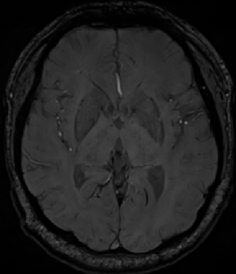
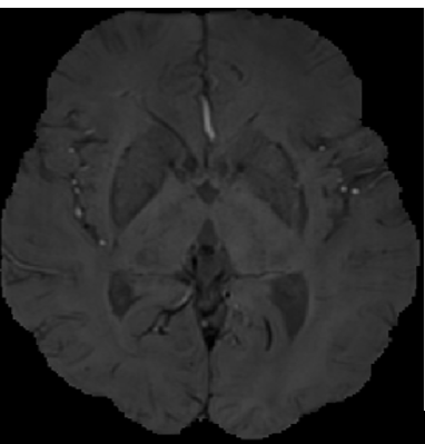
Figure 2. SWI image before skull removal Figure 3. SWI image after skull removal

3.2.Screening stage of microbleeding candidate points based on traditional algorithm

In this paper, a two-stage algorithm is used to detect CMB. In the first stage, candidate points are screened, and in the second stage, candidate points are classified to find out the real microhemorrhagic points, so that no missing detection can occur in the candidate point screening stage. Considering that CMB is a low-frequency signal on SWI images, and according to the morphological characteristics of CMB, it can be seen that CMB presents circular or oval (non-linear) lesions with a diameter of 2-10mm on SWI images. Therefore, this paper adopts the method of fast radial symmetric transformation algorithm combined with threshold segmentation and morphological features to select candidate points, and adopts the method of combining the two methods to avoid the occurrence of missing detection.

3.3.Convolutional neural network implementation

3.3.1.3D convolutional neural networks

The principle of 3D convolutional neural network is to carry out convolution in three-dimensional space through convolution kernel, and the 3D convolution operation can be expressed by formula 1.

\( {V_{xyz}}=f(\sum _{i=1}^{h}\sum _{j=1}^{w}\sum _{k=1}^{d}{w_{ijk}}\cdot {u_{(x+i)(y+i)(z+k)}}+b)\ \ \ (1) \)

In the above formula,\( h \),\( w \), and\( d \)are the dimensions of the convolution kernel\( K \),\( u \)is the image information,\( b \)is the bias, and\( {V_{xyz}} \)is the output after convolution.

3.3.2.Parameter number and computational cost of 3D convolutional neural network

When designing a convolutional neural network, it is usually necessary to consider not only the performance of the network, but also the two important factors, the number of parameters and the calculation cost, which will lead to excessive resource consumption.

Therefore, to calculate the parameter number and computation cost of a convolutional neural network, the parameter number and computation cost of a single convolutional layer need to be calculated first.

The formula for calculating the number of single 3D convolution parameters is as follows:

\( Parmas={C_{out}}×({K_{w}}×{K_{h}}×{K_{d}}×{C_{in}}+1)\ \ \ (2) \)

Where\( {C_{in}} \)is the number of channels of input data,\( {C_{out}} \)is the number of channels of output data, and\( {k_{h}} \),\( {k_{w}} \)and\( {k_{d}} \)are respectively the height and width of the convolution kernel. +1 represents the offset term.

Similarly, the computational cost of a single 3D convolution can be calculated using the following formula:

\( FLOPs=2×({K_{w}}×{K_{h}}×{K_{d}}×{C_{in}})×({C_{out}}×H×W×D)\ \ \ (3) \)

Where\( H \),\( W \)and\( D \)are the height width and depth of the output data respectively.

3.4.Precise identification phase based on deep learning algorithm

The main purpose of this stage is to classify the microhemorrhagic candidates selected in the first stage, so as to distinguish the real microhemorrhagic sites from the similar brain microhemorrhagic analogues. In the first stage, the candidate points with high probability of microbleeding are screened out by the algorithm. Then, in order to reduce the calculation cost, the candidate points selected in the first stage are cut out an image block of 21×21×21 with the candidate point position as the center. This size is adopted because the diameter of microbleeding points is 2~10mm, so the size should not be too small, and the microbleeding points must be surrounded. However, it should not be too large, because too large size may produce too much redundant spatial information, affecting the performance of the model.

4.Analysis of CMB detection results

4.1.Test result evaluation index

CMB detection is a binary classification problem, for which the detection results can be divided into Positive and Negative classes. For the task of CMB detection in this paper, the presence of CMB in the image can be considered as positive (positive class), and the absence of CMB in the image can be considered as false positive (negative class). In the actual test, the following four situations will occur.

Truepositive (TP) : The network predicted CMB, but it was CMB.

There is a Falsepositive (FP) : The network is predicted to be a CMB but is not actually a CMB, a false positive.

Truenegative (TN) : The test is not CMB and is not actually CMB.

Falsenegative (FN) : detects no CMB and is actually CMB, which is a missed detection.

In order to evaluate the performance of the CMB detection method in this paper, Sensitivity (S) and Percision (P) were used to measure the detection effect.

Sensitivity (S), which is Truepositiverate (TPR). It is defined as follows.

\( S=\frac{TP}{TP+FN}\ \ \ (4) \)

The accuracy rate (P), also known as the accuracy rate, represents how many of the predicted positive samples are really positive samples. It is for our predicted results, and its definition is as follows.

\( P=\frac{TP}{TP+FP}\ \ \ (5) \)

The closer the value of the accuracy rate is to 1, the less the number of negative samples are divided into positive samples in the predicted result, that is, the better the classification effect.

The average number of false positives\( F{P_{avg}} \)is defined as follows:

\( F{P_{avg}}=\frac{FP}{N}\ \ \ (6) \)

Where,\( N \)represents the total number of subjects in the test set. The average number of false positives represents the number of false positive samples produced on the average recipient, and the smaller the value, the better the classification effect.

4.2.Data set processing

The dataset used in this paper is a dataset for the detection of cerebral microbleeds, including SWI images and Pha images of 480 patients. The dataset was obtained using the Trio Siemens scanner of 3T, which has the following imaging parameters: Repetition time (TR) is 27ms, echo time (TE) is 20ms, turnover Angle (FA) is 15°, pixel bandwidth (BW) is 120HZ/ pixel, volume size is 512×448×72, layer thickness is 2mm, field of view (FOV) is 256×224mm2, scanning time is 4.45 minutes. The subjects were drawn from two groups; 214 patients were from stroke patients (mean age standard deviation of 68.2±10.1) and 266 were from older adults with normal aging (mean age standard deviation of 70.1±4.0). Data labeling was performed by a neurologist with 24 years of experience and a neurologist with 12 years of experience.

The data set was divided into a training set, a validation set and a test set. As shown in Table 1, the training set contained data from 340 patients, of which 150 were from stroke patients and 190 were from normal aging elderly people. The validation set contained data from 70 patients, 32 of whom were stroke patients and 38 of whom were aging normally. The test set contained data from 70 patients, including 32 from stroke patients and 38 from older adults who were aging normally.

Table 1. Data distribution

4.3.System implementation

This summary mainly introduces the main hyperparameter Settings in the experiment of software and hardware platforms and deep learning algorithms, including weight initialization method, optimization algorithm and learning rate.

4.3.1.Hardware and software platform

All experiments in this paper were conducted on the same hardware device, in which the operating system was Windows 10 and the GPU was NVIDIA GeForce GTX1080Ti. The FRST algorithm and the algorithm based on the combination of threshold segmentation and geometric methods are implemented by Matlab R2018b. Pytorch framework is used for deep learning training, Python is used in programming languages, and common third-party libraries include OpenCV and Numpy.

4.3.2.Weight initialization

He Keming et al. proposed the He initialization method in 2015. He initialization method effectively solves the problem that Xavier initialization performs poorly on ReLU activation functions, and is also a more commonly used initialization method. Random initialization weights are used in this experiment.

4.3.3.Learning rate

The learning rate size controls the updating speed of network weights. If the learning rate is too small, the network convergence speed is slow, time and computing resources are wasted, and overfitting is easy to occur. If the learning rate is set too large, the loss function may oscillate around the minimum value and fail to converge. Therefore, the learning rate is closely related to the performance of the model. In general, there are two ways to set the learning rate. One is the fixed learning rate, which is set to a fixed value and remains unchanged during the whole training process of the network. The other is variable learning rate, which is constantly changing in the iterative process of the network. Usually, a larger learning rate is selected at the initial stage of training to speed up the convergence speed, and with the continuous iteration, the learning rate slowly declines. In the later stage of training, in order to avoid shock, the learning rate will become smaller and smaller. Learning rate attenuation includes exponential attenuation, fixed value attenuation, step by step attenuation, custom attenuation and so on. The method of custom attenuation is adopted in this paper. The initial learning rate is 0.001. Decay 90% every 20 epochs.

4.3.4.Optimization algorithm

The function of the optimization algorithm is to update the parameters in the network according to the learning rate and loss we get. Gradient descent is an optimization algorithm is an optimization algorithm. It is mathematically understandable that the direction function along the gradient grows the fastest, so the opposite direction of the gradient is the direction in which the function falls the fastest. All optimization algorithms in the field of deep learning need to update parameters according to gradient.

4.4.Experimental results of candidate selection stage

In the candidate point screening stage, this experiment conducted candidate point screening based on the FRST algorithm and micro-bleeding candidate point screening based on the combination of threshold segmentation and geometric methods. It can be seen that the candidate point screening based on the combination of threshold segmentation and geometric methods will produce a large number of false positive samples, which will greatly increase the computational load in the subsequent identification stage. It also wastes a lot of computing time. The results of candidate point screening by FRST algorithm remove a large number of false positive samples, and only retain the CMB candidate region with high probability, which greatly reduces the computational load in the subsequent identification stage.

4.4.1.Screening results of microbleeding candidate points based on threshold segmentation and morphological characteristics

The results of the screening method for microbleeding candidate points based on the combination of threshold segmentation and morphological characteristics are shown in Figure 4. Figure a is the SWI image with CMB in a certain layer of patients, Figure b is the label of CMB marked by doctors, and Figure c is the label of CMB screened by threshold segmentation. The D-diagram is the label of the CMB that is finally screened based on the C-diagram and generated by the constraints such as volume and shape. It can be clearly seen from the figure that through morphological features and constraints such as volume, area and shape, it can be seen that many non-circular and non-circular areas have been removed from the processed image.

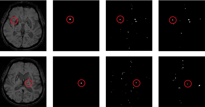
(a) SWI images of patients (b) Doctor's label (c) label for threshold segmentation (d) label after morphological constraint

Figure 4. Threshold segmentation and geometric methods filter the results

4.4.2.Screening results of microbleeding candidate sites based on FRST

Screening results of fast radial and symmetric transformation are shown in Figure 5. Figure a is SWI image with CMB in a certain layer of patients, Figure b is label labeled by doctors, and Figure c is label candidate point of CMB selected by using fast radial and symmetric transformation. The fast radial symmetric transformation algorithm can screen out the candidates of brain microhemorrhagic sites, but there are false positive samples in the candidates of CMB.

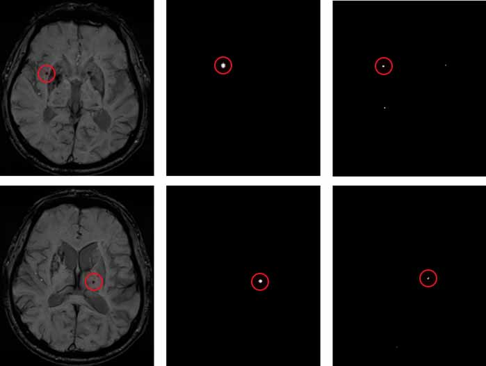
(a) SWI images of patients (b) Doctor's label (c) label generated by the FRST algorithm

Figure 5. FRST algorithm filtering results

4.4.3.The final candidate selection results

As this paper adopts a two-stage cerebral microhemorrhage detection framework, omissions should be avoided during the screening of candidate points in the first stage, that is, the real microhemorrhagic points are not determined as candidate points, which will lead to the failure of the brain microhemorrhagic spot recognition network in the second stage to obtain the missed microhemorrhagic points, resulting in the omission of the entire framework. Therefore, in this paper, the candidate points selected by threshold segmentation and morphological features are fused with the microhemorrhagic points selected by the fast radial transform algorithm, and then input into the recognition network of the second stage.

4.5.Analysis of the results of microbleeding recognition stage

In the recognition stage, the selected candidate points are mainly classified. In the candidate point screening stage, the selected candidate points include a large number of CMB regions and a small number of non-CMB regions, and the 3D convolutional neural network model is trained to recognize the real CMB region.

5.Conclusion

By comparing the experimental results, this paper finds out the most suitable method for screening the candidate points of cerebral microhemorrhagic spot in the first stage. At the same time, the most suitable input size for the second stage is found out through the experiment. Too small input size will lead to incomplete CMB information, and too large input size will lead to excessive redundant information and reduce accuracy. Finally, the type of input data in the identification stage is determined, and the experiment shows that the combination of SWI and Pha can obtain better detection effect.

References

[1]. Yan, Wu, Tao, & Chen. (2016). An up-to-date review on cerebral microbleeds. Journal of stroke and cerebrovascular diseases : the official journal of National Stroke Association, 25(6), 1301-6.
[2]. Haller, S. , Vernooij, M. W. , Kuijer, J. P. A. , Larsson, E. M. , & Barkhof, F. . (2018). Cerebral microbleeds: imaging and clinical significance. Radiology, 287(1), 11-28.
[3]. Haller, S. , Haacke, E. M. , Thurnher, M. M. , & Barkhof, F. . (2021). Susceptibility-weighted imaging: technical essentials and clinical neurologic applications. Radiology, 299(1), 203071.
[4]. Wilson D, Ambler G, Lee KI, Lim IS, Shiozawa M, Koga M, et al. (2019). Cerebralmicrobleeds and stroke risk after ischaemic stroke or transient ischaemic attack: apooled analysis ofindividual patient data from cohort studies. Lancet Neurol, 18:653-665.
[5]. He, K. , Zhang, X. , Ren, S. , & Sun, J. . (2015). Delving deep into rectifiers: surpassing human-level performance on imagenet classification. IEEE Computer Society.
Cite this article
Lv,P. (2024). Research on the precise recognition stage of cerebral microhemorrhage based on deep learning algorithm. Applied and Computational Engineering,88,1-8.
Data availability
The datasets used and/or analyzed during the current study will be available from the authors upon reasonable request.
Disclaimer/Publisher's Note
The statements, opinions and data contained in all publications are solely those of the individual author(s) and contributor(s) and not of EWA Publishing and/or the editor(s). EWA Publishing and/or the editor(s) disclaim responsibility for any injury to people or property resulting from any ideas, methods, instructions or products referred to in the content.
About volume
Volume title: Proceedings of the 6th International Conference on Computing and Data Science
© 2024 by the author(s). Licensee EWA Publishing, Oxford, UK. This article is an open access article distributed under the terms and
conditions of the Creative Commons Attribution (CC BY) license. Authors who
publish this series agree to the following terms:
1. Authors retain copyright and grant the series right of first publication with the work simultaneously licensed under a Creative Commons
Attribution License that allows others to share the work with an acknowledgment of the work's authorship and initial publication in this
series.
2. Authors are able to enter into separate, additional contractual arrangements for the non-exclusive distribution of the series's published
version of the work (e.g., post it to an institutional repository or publish it in a book), with an acknowledgment of its initial
publication in this series.
3. Authors are permitted and encouraged to post their work online (e.g., in institutional repositories or on their website) prior to and
during the submission process, as it can lead to productive exchanges, as well as earlier and greater citation of published work (See
Open access policy for details).