1. Introduction

In the field of financial option pricing, traditional models such as the Black-Scholes [1], Heston [2], Merton Jump-Diffusion [3], and GARCH models [4] have been extensively utilized. The Black-Scholes model is known for its computational simplicity and closed-form solution but is limited by its assumption of constant volatility, which is often unrealistic in financial markets. The Heston model improves upon this by introducing stochastic volatility, which is better in accounting for volatility smiles. The Merton model incorporates jumps in asset prices to capture sudden market fluctuations, and the GARCH model captures volatility clustering in financial time series. However, most of these models have limitations in accurately reflecting real market conditions and require precise parameter estimation.

Recent advancements have integrated machine learning techniques into option pricing, with studies demonstrating the potential of neural networks to model option prices [5]. Machine learning models, including Multi-Layer Perceptrons (MLPs) and Long Short-Term Memory (LSTM) networks, offer flexibility in capturing non-linear relationships and dependencies in financial data [6]. Comparative studies highlight the strengths of traditional models in interpretability and theoretical foundations, while machine learning models excel in predictive power and adaptability [7]. Practical applications of these models include their use in trading strategies, risk management, and portfolio optimization. The GARCH model is widely used for forecasting volatility, and the Merton model is useful for valuing options in volatile markets. Machine learning models have been integrated into algorithmic trading systems to enhance adaptability and optimize trading strategies [8]. Current research trends involve hybrid approaches combining traditional and machine learning models to leverage the strengths of both [9]. Despite the success of traditional models, they have notable limitation, including oversimplification of market dynamics and dependency on accurately estimated parameters. There is a lack of comprehensive evaluations comparing machine learning techniques with traditional models in option pricing, especially considering various performance metrics under different market conditions. Further research is needed to test these models in real-world applications and integrate additional market factors.

This study aims to explore the advantages of machine learning models in option pricing by evaluating various neural network architectures and comparing their performance with traditional methods. The objectives are to assess predictive accuracy, analyze model performance under our specific market conditions, and propose an optimized approach that integrates traditional models with machine learning techniques. This research contributes to the evolving landscape of financial modeling, it sets as an initial attempt aiming to offer more accurate option pricing strategies that benefit financial market stakeholders.

2. Methods

2.1. Data Collection and Preprocessing

In this study, we collected historical stock prices for the FTSE 100 index using the Yahoo Finance API [10] and obtained historical interest rates, specifically the UK government bond yield, from January 1, 2012, to January 1, 2022, from the UK Debt Management Office and the Bank of England. The dataset has a daily frequency, and any missing values were forward-filled using the last available observation to ensure temporal continuity and accuracy in subsequent analyses. The dataset was split into training and testing sets, with the first 8 years of data used for training and the last 2 years reserved for testing. This approach allows us to evaluate the model’s performance on unseen data, ensuring the robustness and generalizability of our findings.

To obtain continuous compounded returns, we calculated the log returns of stock prices:

where r_t represents the log return at time t, P_t is the price at time t, and P_t−1 is the price at the previous time step. Volatility was computed as the annualized standard deviation of log returns, scaled by the square root of 252, which is the approximate number of trading days in a year:

where std(r) is the standard deviation of r. By following these steps, we can ensure that the data was clean, consistent, and ready for the next stages of feature engineering and model implementation. To enhance model predictions, we derived additional features from the raw data: 1. Daily Returns: Calculated as the percentage change in closing prices to capture daily fluctuations. 2. Volatility: Computed as the rolling standard deviation of returns over a 20-day period to capture recent volatility trends. 3. 20-Day Simple Moving Average (SMA): Calculated as the mean of the past 20 closing prices to highlight longer-term trends and smooth short-term fluctuations. 4. Bollinger Bands: Constructed using the 20-day SMA and standard deviation to identify potential overbought or oversold conditions.

These features, along with the opening price, highest price, lowest price, closing price, and trading volume, were used to provide a comprehensive view of market conditions. The dataset, with these engineered features, was normalized for model training and evaluation. The target variable was the payoff of a European call option, calculated as:

Payoff = max(S_T − K,0) ,

where S_T is the closing price at maturity and K is the strike price, set at 7000. The fixed strike price was chosen to streamline the analysis and focus on a specific scenario for more controlled and detailed insights. This setup resulted in the options being out-of-the-money (OTM) from April 2020 to April 2021, as shown in Figures 1 and 2. OTM options typically have wider bid-ask spreads and provide less information about future volatility, which is a known limitation. Nevertheless, this approach allows us to systematically explore the model's performance under our specific set of conditions.

2.2. Models for Predicting Option Prices

We applied several math models to predict option prices, including the Black-Scholes, GARCH, Heston, and Merton Jump-Diffusion, each offering unique approaches to capturing market dynamics and volatility. It is crucial to estimate the parameters of each model accurately. For example, in the GARCH model, parameters such as Omega, Alpha, and Beta are estimated using maximum likelihood estimation (MLE). For the Heston and Merton models, parameters like volatility, mean-reversion rate, and jump intensity are estimated based on historical data. However, it is important to note that assuming future prices will have the same volatility as historical prices is often questionable. Market practitioners prefer using implied volatility derived from current market prices of options, as it more accurately reflects the market's expectations of future volatility, which worths to be further investigated in future works.

The value of an option under a risk-neutral probability measure is determined by:

${C_{t}}={B_{t}}{E_{}}(\frac{{C_{T}}}{{B_{T}}}|{F_{t}})$

where B_tis the discount factor [11]. For practical implementation, the option value at the initial time t = 0 is calculated as:

${C_{0,i}}=exp{(-{r_{T}})}{C_{T,i}}$

Here, r is the risk-free interest rate, T is the time to maturity, and C_T,irepresents the payoff at maturity for the i-th simulation. Averaging the outcomes from N simulations yields the option price estimate:

${\hat{C}_{0}}=\frac{1}{N}\sum _{i=1}^{N}{C_{0,i}}$

Monte Carlo simulations were employed for models where closed-form solutions are complex or non-existent, such as the Heston model and the Merton Jump-Diffusion model. These models involve stochastic processes with features like stochastic volatility or jumps, which lack straightforward analytical solutions. Monte Carlo methods enable flexible and accurate pricing by simulating numerous possible paths for the underlying asset prices and averaging the resultant payoffs. For fairness in performance comparisons, we matched the simulation methods to each model's characteristics. The Heston model benefits from Monte Carlo simulations to capture its path-dependent nature and volatility dynamics accurately. Similarly, the Merton model relies on simulations to account for sudden price jumps and simulate realistic price paths. In contrast, the Black-Scholes and GARCH models were evaluated using MLE, which optimally estimates parameters based on observed data, minimizing bias from numerical approximations and avoiding the computational intensity of simulations. This approach ensures that the performance of these models is assessed based on fitting historical volatility patterns.

To enhance the accuracy of Monte Carlo simulations for models like Heston and Merton, we employed variance reduction techniques such as Antithetic Variates and Control Variates. These methods reduce simulation variance, leading to more reliable estimates with fewer runs [11]. Combining these techniques with a sufficiently large number of simulations (100,000) ensures that our comparisons reflect the true predictabilities of each model while capturing the complexities of financial markets.

Table 1. Model Performance with Error Metrics Formulas

$MSE=\frac{1}{n}\sum _{i=1}^{n}{({y_{i}}-\hat{{y_{i}}})^{2}}$

$MAE=\frac{1}{n}\sum _{i=1}^{n}|{y_{i}}-\hat{{y_{i}}}|$

$RMSE=\sqrt[]{\frac{1}{n}\sum _{i=1}^{n}{({y_{i}}-\hat{{y_{i}}})^{2}}}$

${R^{2}}=1-\frac{\sum _{i=1}^{n}{({y_{i}}-\hat{{y_{i}}})^{2}}}{\sum _{i=1}^{n}{({y_{i}}-\bar{y})^{2}}}$

3. Results

Table 1 shows that the GARCH model leads in performance with the lowest MSE, MAE, RMSE, and CV MSE, and the highest R² value, indicating its strong ability to capture volatility clustering. The Tuned Neural Network also performs well, with low error metrics and a high R² value, demonstrating its effectiveness in managing complex non-linear relationships. Machine learning models like Random Forest, Gradient Boosting, and LSTM also show strong results. In contrast, traditional models like Merton, Black-Scholes, and Heston have higher errors and lower R² values, with the Merton model particularly struggling with sudden jumps and complex dynamics. Linear Regression shows high errors, highlighting the benefits of more sophisticated models.

(a) (b)

(c) (d)

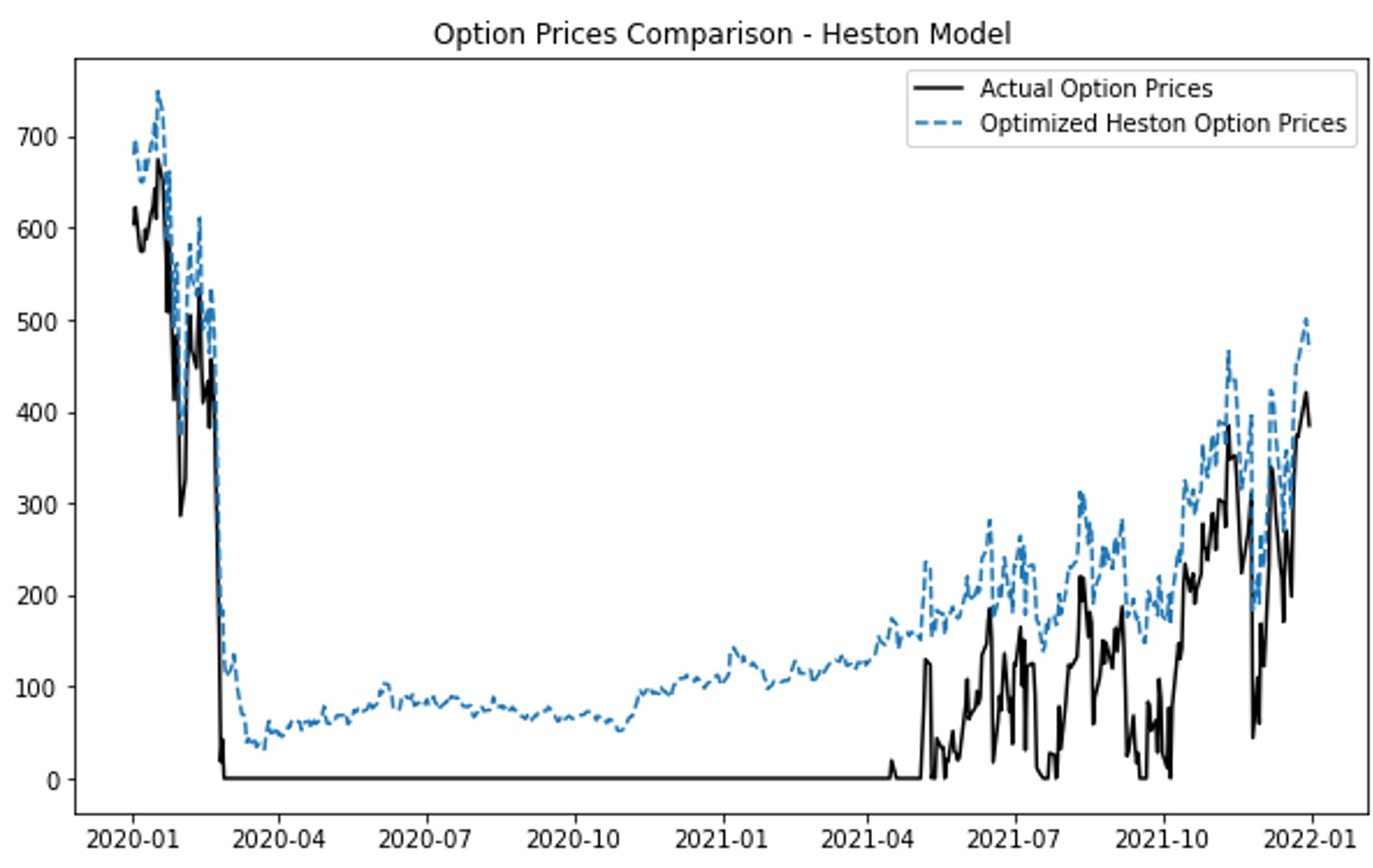
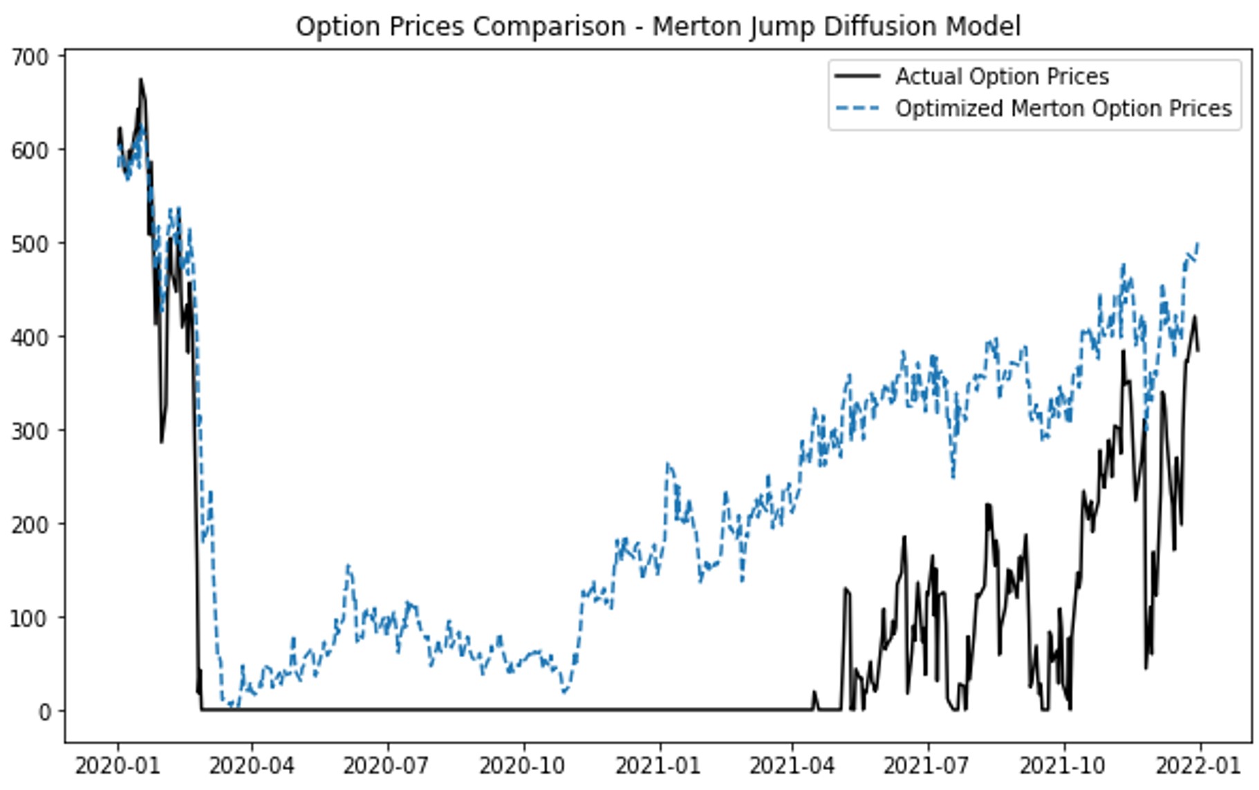
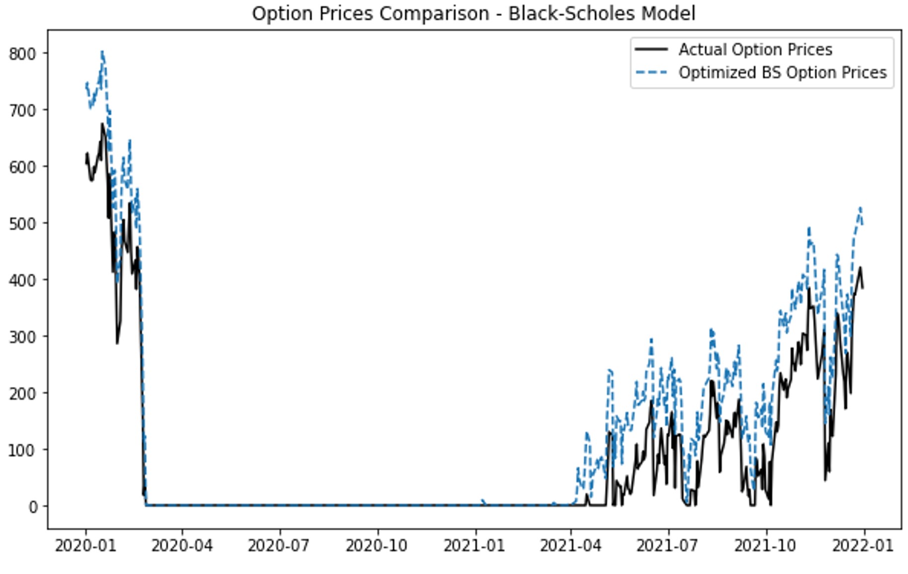
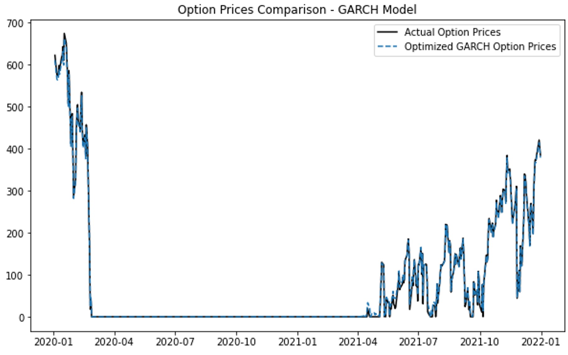
Figure 1. Option Prices Comparison: (a) Black-Scholes Model; (b) GARCH model; (c) Heston Model; (d) Merton Jump Diffusion Model

Figure 1(a) shows that the Black-Scholes model predicts option prices accurately during stable periods but fails to account for volatility spikes, leading to significant deviations during high volatility periods like early-2020 and mid-2021. Figure 1(b) demonstrates that the GARCH model aligns closely with actual prices, effectively capturing market volatility and providing reliable predictions even during turbulent periods. In Figure 1(c), the Heston model captures stochastic volatility but shows discrepancies during volatile periods, suggesting it may not fully handle market instability. Figure 1(d) reveals that the Merton Jump Diffusion model effectively captures price jumps but tends to overestimate during stable periods, indicating its sensitivity to sudden market changes and a need for improved calibration.

(a) (b)

(c) (d)

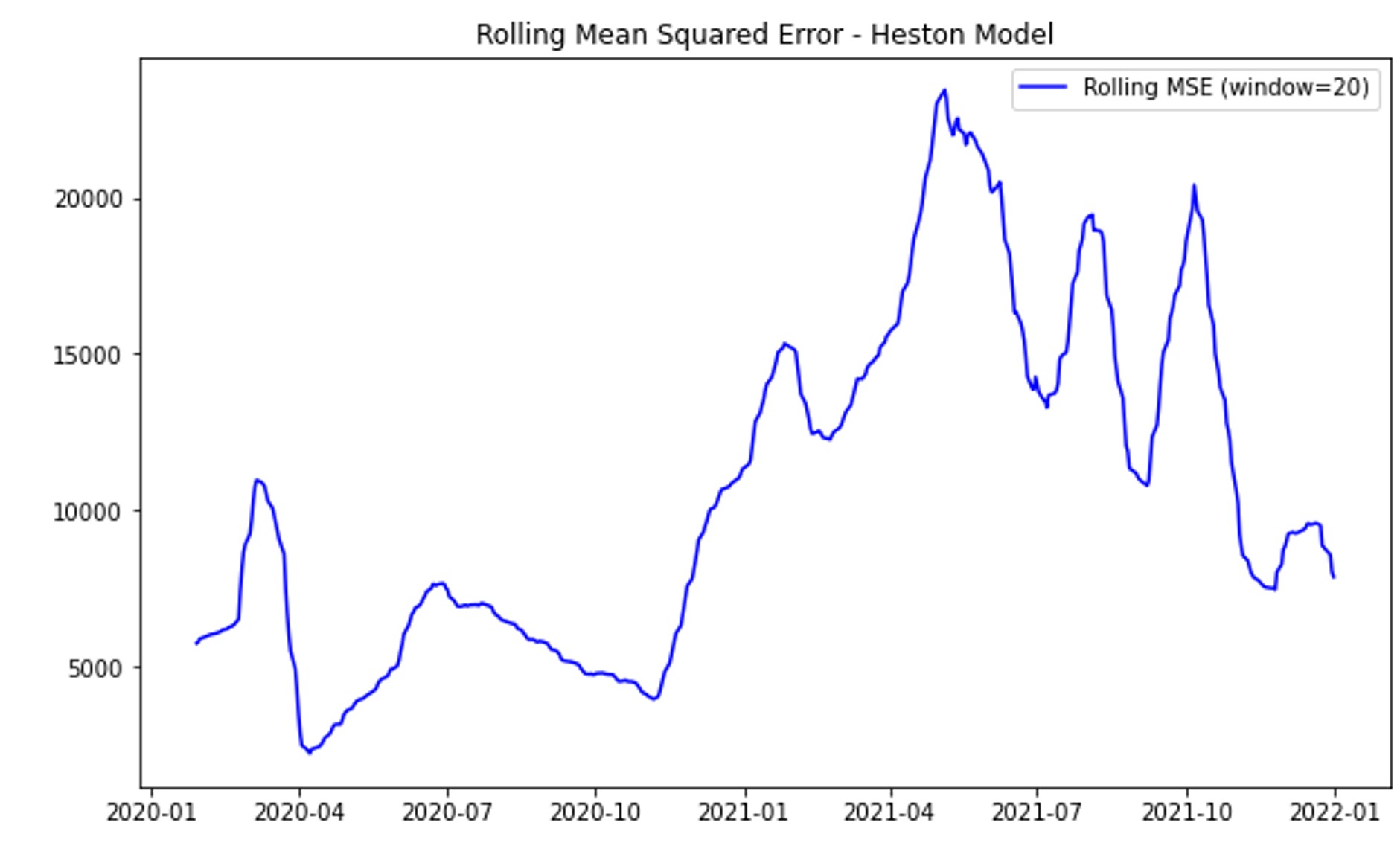
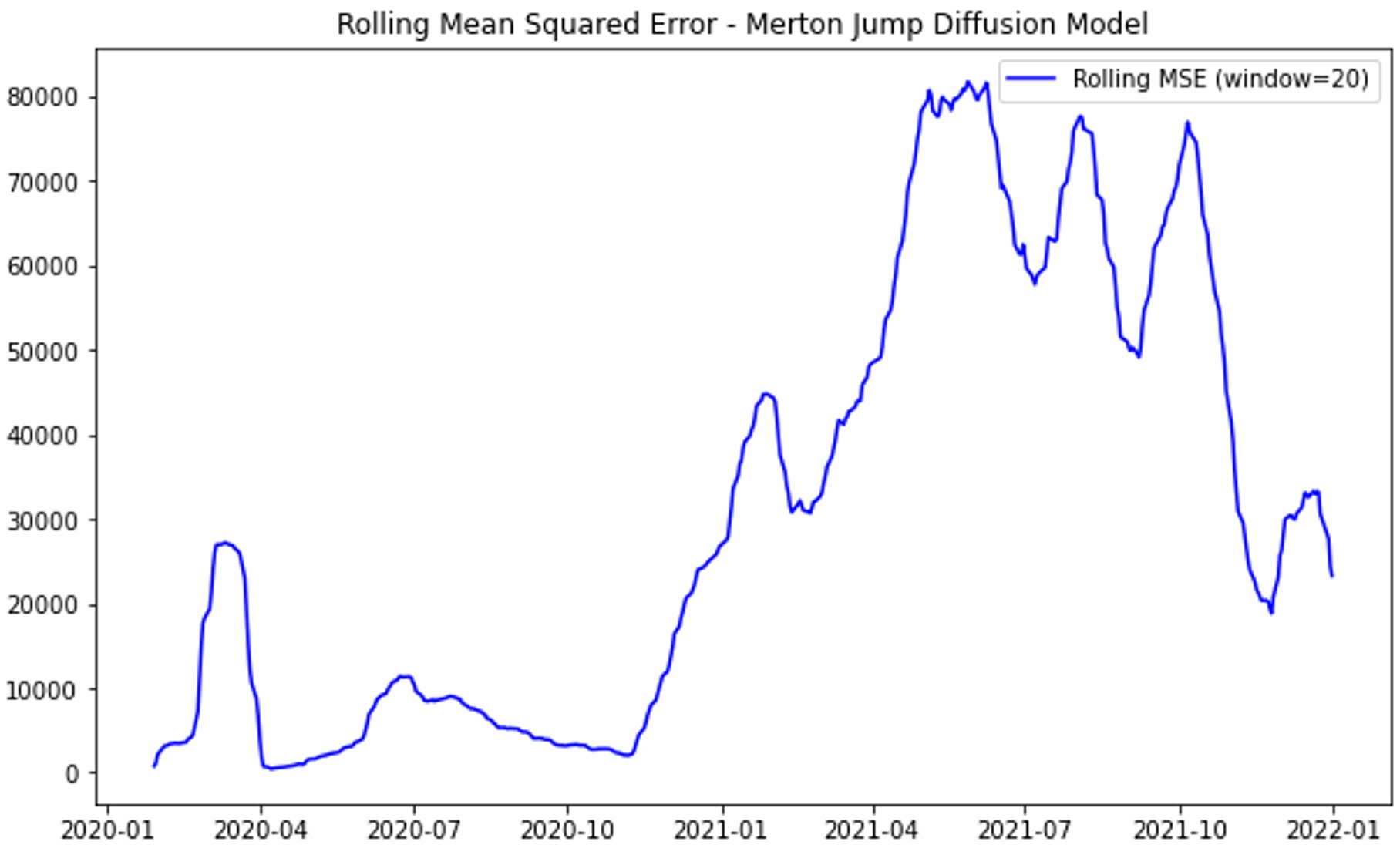
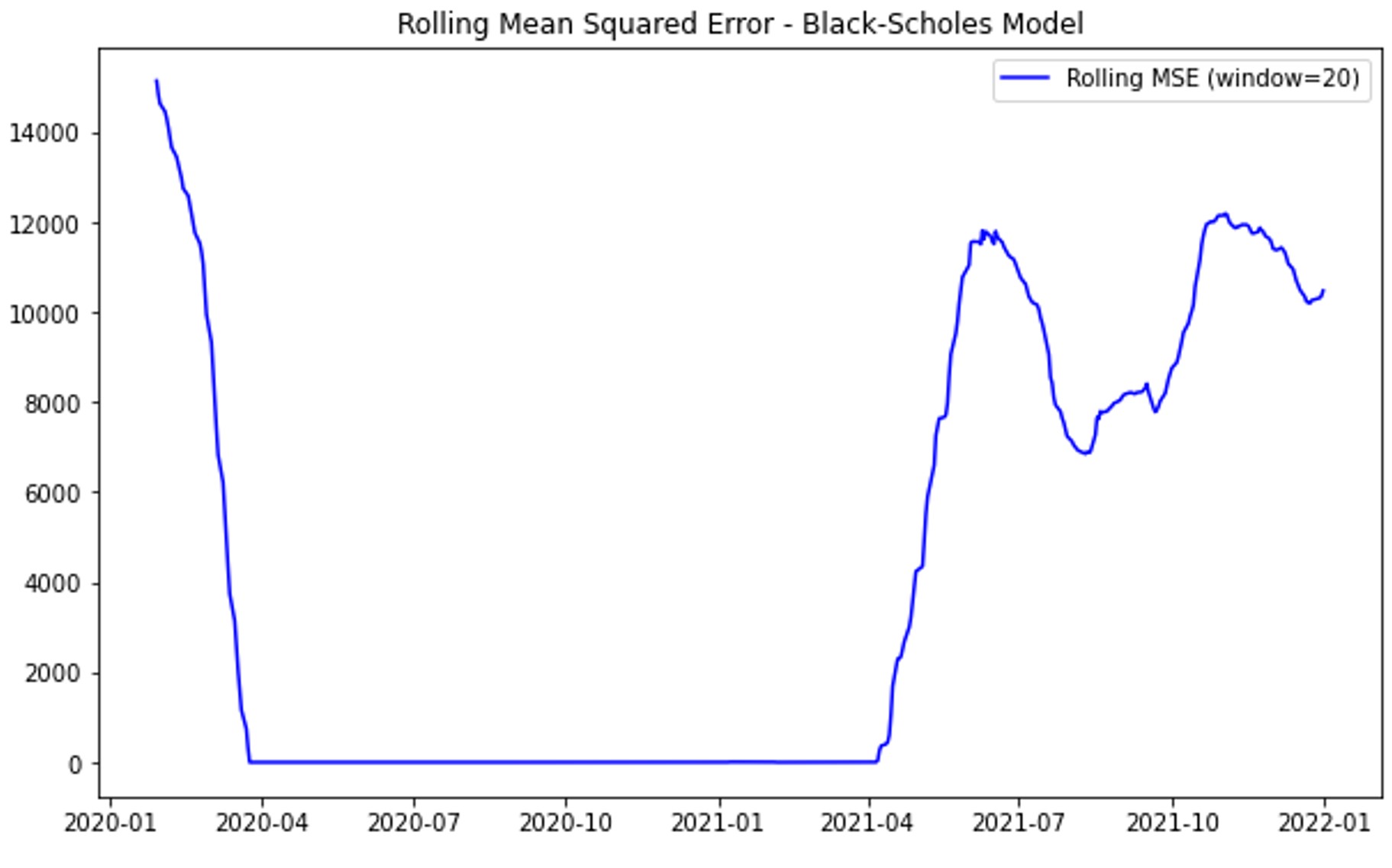
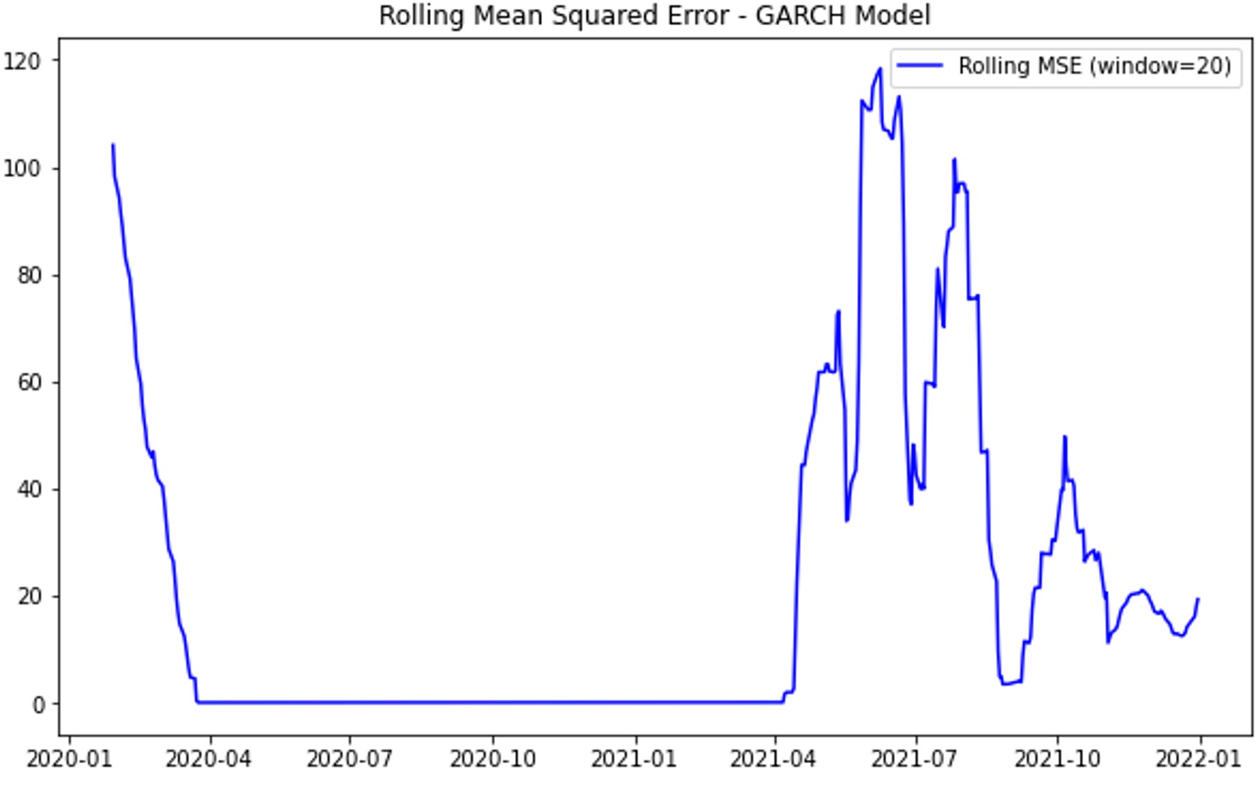
Figure 2. Rolling Mean Squared Error (MSE): (a) Black-Scholes Model; (b) GARCH model; (c) Heston Model; (d) Merton Jump Diffusion Model

Figure 2(a) shows that the Black-Scholes model's rolling mean squared error (MSE) remains stable during calm periods but spikes significantly during volatile times, such as early-2020 and mid-2021, due to its constant volatility assumption. Figure 2(b) illustrates that the GARCH model maintains low MSE with only minor spikes during extreme volatility, reflecting its robustness in capturing market dynamics and volatility clustering. Figure 2(c) reveals that the Heston model has higher MSE during volatile periods, indicating limitations in handling sudden market changes despite accounting for stochastic volatility. Figure 2(d) shows that the Merton Jump Diffusion model struggles with accuracy in both volatile and stable periods, with consistently high MSE and significant spikes during market turbulence. This consistent poor performance highlights the Merton model's inadequacy in capturing market dynamics accurately across varying conditions.

4. Discussion

4.1. Interpretation of Findings

The results of this study provide significant insights into the predictabilities of various models for option pricing. The GARCH model emerged as the most effective, consistently outperforming other models across multiple performance metrics. Its lowest MSE, MAE, RMSE, and CV MSE, along with the highest R² value, indicate its superior accuracy and robustness in capturing volatility clustering in financial markets. This finding aligns with the inherent design of the GARCH model, which effectively models time-varying volatility, a common characteristic in financial data. The GARCH model’s ability to dynamically adjust to changes in market volatility makes it particularly suited for options pricing, where accurate volatility prediction is crucial. The Tuned Neural Network also demonstrated strong performance, showcasing the effectiveness of optimized hyperparameter tuning in managing complex non-linear relationships. Its ability to capture intricate patterns in data underscores the potential of machine learning techniques in financial modeling. The strong performance of other machine learning models like Random Forest, Gradient Boosting, and LSTM further confirms their capability to handle the non-linearities and dependencies in financial datasets, making them valuable tools for option pricing.

In contrast, traditional models such as the Merton, Black-Scholes, and Heston models showed higher errors and lower R² values. Which indicates their respective limitations in predicting option prices under market conditions which differ from their theoretical assumptions. The Merton model exhibited the highest errors and the lowest R² value, reflecting its struggle to capture sudden jumps and complex market dynamics effectively. While traditional models have a solid theoretical foundation, they may not be as adaptable to the nuances of real-world financial data as more flexible machine learning models.

4.2. Comparison with Previous Studies

Our findings mostly align with previous studies that emphasize the superiority of advanced ML models in capturing market complexities. Ruf and Wang [5] demonstrated the potential of neural networks in modeling option prices, and our results further corroborate their conclusions by showing the strong performance of the Tuned Neural Network. This consistency indicates that machine learning models, when properly tuned, can provide significant advantages over almost all traditional models in terms of predictive accuracy and adaptability.

Similarly, the limitations of traditional models, as highlighted in studies by Feng et al. [7], are evident in our findings. The Black-Scholes model, despite its widespread use, underperformed compared to machine learning approaches. This is consistent with the literature that criticizes the Black-Scholes model for its assumption of constant volatility, which is often unrealistic in financial markets. The Heston model, although introducing stochastic volatility, also showed limitations, particularly during periods of high market volatility. Our study supports the notion that while these models have theoretical elegance, their practical application may be limited by their underlying assumptions.

The performance of the GARCH model in our study aligns with the findings of Bollerslev [4], who highlighted the model’s effectiveness in capturing volatility clustering. This reinforces the importance of using models that can adapt to changing market conditions. Additionally, the strong performance of the Tuned Neural Network and other machine learning models echoes the findings of Hutchinson et al. [12], who first proposed using neural networks for option pricing, demonstrating their potential to surpass traditional models.

5. Conclusion

The GARCH model exhibits the lowest error metrics and the highest R² value, highlighting its forte in capturing volatility clustering. Machine learning models, particularly the Tuned Neural Network, also demonstrate strong predictabilities, effectively managing complex non-linear relationships in financial data. In contrast, traditional models like the Black-Scholes, Heston, and Merton Jump-Diffusion models show higher errors and lower R² values, reflecting their limitations in handling real-world market dynamics. Based on our comparative results, we hypothesize that an ensemble model combining our Tuned Neural Network and the GARCH model could further enhance predictive accuracy. To validate this hypothesis, we constructed an ensemble model that integrates the strengths of both approaches. Due to page constraints, detailed results of this ensemble model are not included here. Interested readers are welcome to email me for access to this supplementary material. Future works will consider using at-the-money (ATM) options and varying strike prices to better capture the implied volatility smile.

For those interested in a more comprehensive exploration, the extended version of this research includes a detailed literature review of traditional models and their recent advancements, a thorough discussion on research gaps and limitations of these models under varying market conditions, and in-depth descriptions of feature engineering and data preprocessing techniques used in the study. It also covers extensive descriptions of mathematical models with their equations and parameter estimations, the implementation of Monte Carlo simulations for complex models like Heston and Merton, detailed implementation and hyperparameter tuning of machine learning models, and a comprehensive set of results with comparison tables, figures illustrating model performance metrics, rolling MSE, and model loss plots. Additionally, the extended version includes a sensitivity analysis of model parameters and their impact on predictive accuracy. Readers interested in these detailed sections, comparisons, and figures can email me for access to the extended versions of this research as well as future work, or alternatively, contact me via ResearchGate. Welcome for any discussion, suggestions or corrections!

References

[1]. Black, F., & Scholes, M. (1973). The Pricing of Options and Corporate Liabilities. Journal of Political Economy, 81(3), 637-654.
[2]. Heston, S. L. (1993). A Closed-Form Solution for Options with Stochastic Volatility with Applications to Bond and Currency Options. Review of Financial Studies, 6(2), 327–343. Oxford University Press.
[3]. Merton, R. C. (1976). Option Pricing When Underlying Stock Returns Are Discontinuous. Journal of Financial Economics, 3(1-2), 125–144. Elsevier.
[4]. Bollerslev, T. (1986). Generalized autoregressive conditional heteroskedasticity. Journal of Econometrics, 31(3), 307-327.
[5]. Ruf, J., & Wang, W. (2020). Neural Networks for Option Pricing. Quantitative Finance, 20(9), 1539.
[6]. Zhang, W., Li, Z., & Zhu, Q. (2019). Stock Price Prediction via Convolutional Neural Networks. Proceedings of the IEEE Conference on CVPR Workshops, 2555–2562.
[7]. Feng, G., Giglio, S., & Xiu, D. (2018). Deep Learning in Asset Pricing. Review of Financial Studies, 33(5), 2223-2273.
[8]. Fischer, T., & Krauss, C. (2018). Deep Learning With Long Short-Term Memory Networks for Financial Market Predictions. European Journal of Operational Research, 270(2), 654–669.
[9]. Liu, Q., Wang, Z., & Li, X. (2019). A Hybrid Framework for Option Pricing Combining Machine Learning and Parametric Models. Journal of Financial Economics, 134(3), 706–725.
[10]. Yahoo Finance. (2023). Stock Market Data. Retrieved from https://finance.yahoo.com.
[11]. Glasserman, P. (2004). Monte Carlo Methods in Financial Engineering (Vol. 53). Springer Science & Business Media.
[12]. Hutchinson, J. M., Lo, A. W., & Poggio, T. (1994). A Nonparametric Approach to Pricing and Hedging Derivative Securities Via Learning Networks. Journal of Finance, 49(3), 851-889.
Cite this article
Wang,Z. (2024). Comparative analysis of machine learning and traditional models for financial option pricing. Applied and Computational Engineering,88,174-181.
Data availability
The datasets used and/or analyzed during the current study will be available from the authors upon reasonable request.
Disclaimer/Publisher's Note
The statements, opinions and data contained in all publications are solely those of the individual author(s) and contributor(s) and not of EWA Publishing and/or the editor(s). EWA Publishing and/or the editor(s) disclaim responsibility for any injury to people or property resulting from any ideas, methods, instructions or products referred to in the content.
About volume
Volume title: Proceedings of the 6th International Conference on Computing and Data Science
© 2024 by the author(s). Licensee EWA Publishing, Oxford, UK. This article is an open access article distributed under the terms and
conditions of the Creative Commons Attribution (CC BY) license. Authors who
publish this series agree to the following terms:
1. Authors retain copyright and grant the series right of first publication with the work simultaneously licensed under a Creative Commons
Attribution License that allows others to share the work with an acknowledgment of the work's authorship and initial publication in this
series.
2. Authors are able to enter into separate, additional contractual arrangements for the non-exclusive distribution of the series's published
version of the work (e.g., post it to an institutional repository or publish it in a book), with an acknowledgment of its initial
publication in this series.
3. Authors are permitted and encouraged to post their work online (e.g., in institutional repositories or on their website) prior to and
during the submission process, as it can lead to productive exchanges, as well as earlier and greater citation of published work (See
Open access policy for details).