1. Introduction

As global climate change intensifies, accurate weather forecasting becomes increasingly crucial in agriculture, energy management, environmental protection, and daily life. Weather prediction accuracy directly impacts socio-economic development and quality of life. Traditional methods, which primarily rely on physical models and statistical approaches, face limitations in handling complex nonlinear and time-varying features, especially under the increased uncertainty brought by climate change [1].

In recent years, deep learning techniques have shown strong potential in weather prediction, particularly in managing complex nonlinear relationships and time series data [2]. For instance, Convolutional Neural Networks (CNN) effectively capture spatial patterns in weather data, while Recurrent Neural Networks (RNN) and Long Short-Term Memory Networks (LSTM) excel in processing meteorological time series, capturing time-dependence in variables [3]. Despite significant progress in areas like rainfall and temperature trend prediction, single models struggle with high-dimensional, multi-scale weather data. Consequently, researchers are exploring hybrid models combining CNN and LSTM to enhance weather prediction performance [4]. This paper focuses on analyzing and predicting historical temperature data in Delhi, India, using a CNN-LSTM hybrid model. We conducted comprehensive data preprocessing and exploratory analysis, followed by constructing and training the model. The experimental results demonstrate the model’s strong performance in prediction accuracy and stability, highlighting its potential in weather forecasting. This research provides insights into the effectiveness of the CNN-LSTM model in meteorological time series data and supports the broader application of deep learning in weather prediction.

2. Related Work

In time series forecasting, traditional models like Autoregressive Moving Average (ARMA) and Autoregressive Integrated Moving Average (ARIMA) have long been standard due to their effectiveness in handling linear and stationary data. These models, along with Exponential Smoothing, have seen extensive use in fields such as economic forecasting and energy consumption prediction, particularly with stable, cyclical data [1]. However, their linear assumptions limit their performance when dealing with nonlinear, complex, and time-varying data [2, 3].

The advent of Recurrent Neural Networks (RNNs) and Long Short-Term Memory (LSTM) networks addressed some of these limitations by capturing long-term dependencies in sequential data, proving effective in domains like speech recognition and text generation [3, 4]. Despite their strengths, LSTMs may struggle with intricate local patterns and can be prone to overfitting, especially with limited data or noisy feature [5].Conversely, Convolutional Neural Networks (CNNs), originally dominant in computer vision, have shown promise in feature extraction from one-dimensional time series data. Their application to time series classification, such as ECG signal classification, has demonstrated significant accuracy improvements [6].

To address these issues, hybrid models combining CNNs and LSTMs have been developed, leveraging CNN's local pattern recognition with LSTM's temporal modeling capabilities. This CNN-LSTM architecture has shown effectiveness in tasks like precipitation forecasting, offering improved accuracy and robustness across varying conditions [7]. However, these models also introduce increased computational complexity and risk of overfitting, especially with high-dimensional or noisy data [4].

In weather forecasting, particularly in regions with complex climates like Delhi, deep learning models have been increasingly employed for predicting elements such as temperature, rainfall, and wind speed [8]. This study focuses on developing a CNN-LSTM model for temperature forecasting in Delhi, aiming to capture the complex patterns in the region’s climate data more effectively than existing methods. The model's performance will be evaluated using metrics like MSE, with discussions on potential challenges such as overfitting and computational demands.

3. Prediction Model

3.1. Dataset

The dataset used in this study is the Delhi Temperature Dataset, containing temperature records over a specified period, recorded daily or hourly. It includes features like temperature and weather conditions. The training set consists of 7,300 samples, covering around 20 years of historical data, used to train the CNN-LSTM model for temperature prediction.

3.2. Data Preprocessing

Data preprocessing is a critical step in model training. When creating time series data, it was standardized to the range of [-1, 1] using the MinMaxScaler, a method widely recognized for its effectiveness in normalizing data [1]. The mathematical formula is as follows.

\( {x^{ \prime }}=2\cdot \frac{x-min{(x)}}{max{(x)}-min{(x)}}-1 \) (1)

This step accelerated the model's convergence. Initially, the temperature data is normalized to ensure that all features are on the same scale. We apply Min-Max normalization, scaling the data to a range between -1 and 1, which accelerates model training and improves convergence. Next, missing values in the dataset are addressed, either by imputing with the mean of the corresponding column or by removing the affected samples [2]. Additionally, feature engineering is performed to generate time-related features (e.g., season, month) that enhance the quality of the input data for the model [5].

3.3. CNN-LSTM Model

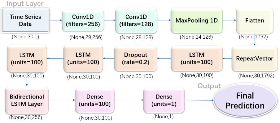Figure 1. Structure of CNN-LSTM Model

The proposed model combines the strengths of one-dimensional convolutional neural networks and long short-term memory networks (LSTM) to predict future temperatures. This architecture in Figure 1 effectively captures both local features [6] and long-term dependencies [3] in time series data, enhancing prediction accuracy. The structure’ s parameters are presented in Table 1.

Table 1. All the layers with specific parameters.

Convolutional Layer

The first Conv1D layer employs 256 convolutional filters, each with a kernel size of 2. Utilizing the ReLU activation function, this layer introduces non-linearity to the model, allowing it to efficiently extract local features from the input sequence. The input consists of 30-time steps, each containing one feature, making this layer crucial for capturing initial patterns in the data. The second Conv1D layer continues the feature extraction process with 128 convolutional filters. By further refining and extracting higher-level features, the ReLU activation function ensures the model's ability to capture more complex patterns within the time series data.

RepeatVector Layer

Next, the RepeatVector layer duplicates the flattened feature vector 30 times. This repetition ensures that the features extracted from the previous layers are available at each time step in the subsequent LSTM layers, facilitating the model’s ability to learn and process temporal dependencies effectively.

Bidirectional LSTM Layer

The model features a series of LSTM layers designed to capture complex temporal dependencies within the input sequence. The initial LSTM layer, with 100 units, captures long-term dependencies and returns outputs for each time step, which subsequent layers build upon. To prevent overfitting, a Dropout layer is applied, randomly dropping 20% of neurons during training. Additional stacked LSTM layers further enhance the model's ability to understand intricate patterns in the data. A Bidirectional LSTM layer is also included, processing data in both forward and backward directions to capture dependencies from both perspectives, thereby improving predictive performance

3.4. Model Training and Optimization

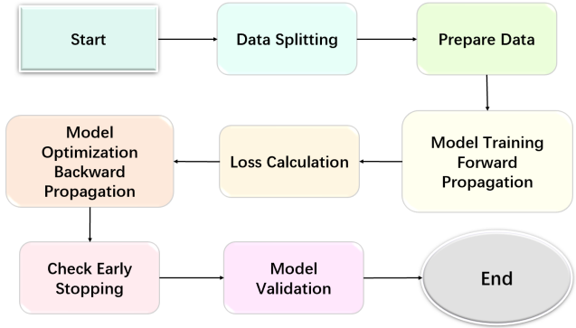
Figure 2. Process of model training and optimization

The model training process (see Figure 2) begins with splitting the dataset into training and testing sets to ensure the model's generalization ability. Typically, the data is divided proportionally, allowing the model to be validated on unseen data. In this study, the temperature data from the previous 30 days is used to predict the temperature of the next day. The training steps include forward and backward propagation from equation (1) (2) (3) and (4), where the model parameters are adjusted by minimizing the loss function \( L(θ) \) . EarlyStopping callback is employed to halt training when the training loss does not decrease over seven consecutive epochs, thereby preventing overfitting.

\( \begin{matrix}{ m _{t}}={β_{1}}{m_{t-1}}+(1-{β_{1}}){∇_{θ}}L({θ_{t}}) (2) \\ {v_{t}}={β_{2}}{v_{t-1}}+(1-{β_{2}}){({∇_{θ}}L({θ_{t}}))^{2}} (3) \\ {\hat{m}_{t}}=\frac{{m_{t}}}{1-β_{1}^{t}}, {\hat{v}_{t}}=\frac{{v_{t}}}{1-β_{2}^{t}} (4) \\ {θ_{t+1}}={θ_{t}}-η\frac{{\hat{m}_{t}}}{\sqrt[]{{\hat{v}_{t}}}+ϵ} (5) \\ \end{matrix} \)

Where: \( {m_{t}} \) and \( {v_{t}} \) are the first and second moment estimates., \( {β_{1}} \) and \( {β_{2}} \) are the exponential decay rates for these estimates., \( η \) is the learning rate., \( ϵ \) is a small constant to prevent division by zero.

4. Results

A. Loss Functions

The choice of loss function has a significant impact on the prediction accuracy of the model. In this experiment, we use both Mean Squared Error (MSE) and Root Mean Squared Error (RMSE) from equation (6) and (7) as loss functions below to evaluate the model's performance. MSE is commonly used to measure the discrepancy between predicted and actual values [7], making it suitable for tasks where we aim to minimize large errors. RMSE, on the other hand, provides a more interpretable metric by taking the square root of MSE, which puts more emphasis on larger errors. The combination of these two loss functions [8] helps in obtaining a more robust evaluation of the model's predictive capabilities. Recent studies [9], [10], and [11] support the effectiveness of these methodologies in various temperature prediction tasks.

\( MSE=\frac{1}{n}\sum _{i=1}^{n} {({y_{i}}-{\hat{y}_{i}})^{2}} (6) \)

\( RMSE=\sqrt[]{MSE} (7) \)

B. Model Training Strategy

During model training, hyperparameters such as learning rate \( η \) and batch size \( B \) are fine-tuned to optimize the model's performance. The learning rate \( {η_{t}} \) can be dynamically adjusted using learning rate schedules in equation (8).

\( {η_{t}}={η_{0}}\cdot \frac{1}{1+ decay \cdot t} (8) \)

The training process begins with an initial learning rate, denoted as \( {η_{0}} \) , and a decay factor applied over time, where \( t \) represents the current epoch or iteration. The maximum number of training epochs, \( T \) , is set to 300. However, this number may be reduced through an early stopping mechanism. Early stopping is triggered if the validation loss ( \( {L_{val }} \) ) fails to improve over a predefined number of epochs, known as the patience period ( \( p \) ). Specifically, training is halted if \( {L_{val }} \) at epoch \( t \) is greater than the minimum \( {L_{val }} \) observed during the previous \( p \) epochs. Throughout the training process, detailed logs are maintained to monitor progress.

C. Model Performance Evaluation

We plot the change curve of the loss function during the training process to observe the model's convergence. The results indicate that both loss functions decrease rapidly in the early stage of training and then stabilize, suggesting that the model successfully learns the patterns in the data, which improves the prediction accuracy.

To comprehensively evaluate the model's performance, we calculate the mean square error (3.26217) and root mean square error (1.80615). The results demonstrate that the CNN-LSTM model performs well on these metrics, with high prediction accuracy and stability. The prediction curve's high similarity to the test curve further supports the model's effectiveness in temperature prediction.

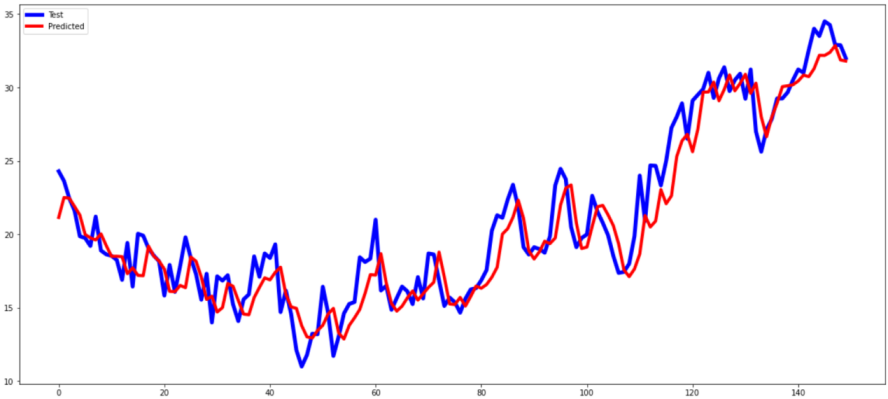
Figure 3. The prediction curve and test curve.

5. Conclusion

In this study, we employed an optimized CNN-LSTM model to predict temperature time series in Delhi, India. The model effectively captures complex spatio-temporal features, significantly improving prediction accuracy. By thoroughly preprocessing and analyzing historical meteorological data from 1996 to 2017, the CNN-LSTM model leverages the feature extraction capabilities of CNNs and the time series processing strengths of LSTMs. The results show that our model outperforms traditional time series prediction methods, offering higher accuracy and stability.However, the study acknowledges certain limitations, such as the need to improve prediction accuracy under extreme weather conditions and enhance dataset representativeness. Future research should focus on optimizing the model architecture, exploring better feature extraction techniques, and applying the model to a broader range of time series forecasting tasks. Additionally, addressing computational complexities and overfitting through regularization techniques will be crucial for improving model stability and generalization.

In summary, this research offers an effective methodology for temperature prediction in Delhi and lays the groundwork for future investigations in related areas, with the CNN-LSTM framework expected to advance multi-disciplinary time series forecasting applications.

References

[1]. E. Kalnay et al., "The NCEP/NCAR 40-Year Reanalysis Project," Bull. Amer. Meteor. Soc., vol. 77, no. 3, pp. 437-471, 1996.
[2]. Y. LeCun, Y. Bengio, and G. Hinton, "Deep learning," Nature, vol. 521, pp. 436-444, 2015.
[3]. S. Hochreiter and J. Schmidhuber, "Long short-term memory," Neural Comput., vol. 9, no. 8, pp. 1735-1780, 1997.
[4]. Y. Qin et al., "A dual-stage attention-based recurrent neural network for time series prediction," in Proc. 26th Int. Joint Conf. Artif. Intell., 2017, pp. 2627-2633.
[5]. F. A. Gers, J. Schmidhuber, and F. Cummins, "Learning to forget: Continual prediction with LSTM," Neural Comput., vol. 12, no. 10, pp. 2451-2471, 2000.
[6]. M. Kiranyaz, T. Ince, and M. Gabbouj, "Real-time patient-specific ECG classification by 1-D convolutional neural networks," IEEE Trans. Biomed. Eng., vol. 63, no. 3, pp. 664-675, Mar. 2016.
[7]. X. Shi et al., "Convolutional LSTM network: A machine learning approach for precipitation nowcasting," in Proc. 29th Conf. Neural Inf. Process. Syst., 2015, pp. 802-810.
[8]. R. Chevallier et al., "Global real-time precipitation forecasting with a neural network approach," in Proc. IEEE Int. Conf. Big Data (Big Data), 2018, pp. 3849-3858.
[9]. A. Ahmed and J. A. S. Alalana, "Temperature prediction using LSTM neural network," in Proc. IEEE 9th International Conference on Electronics (ICEL), 2020, pp. 210-215.
[10]. H. Wang et al., "Temperature forecasting using deep learning methods: A comprehensive review," Energy Reports, vol. 6, pp. 232-245, 2020.
[11]. Y. Zhang et al., "Time series temperature forecasting with convolutional neural networks," in Proc. IEEE International Conference on Data Mining, 2019, pp. 734-739.
Cite this article
Li,B.;Qian,Y. (2024). Weather prediction using CNN-LSTM for time series analysis: A case study on Delhi temperature data. Applied and Computational Engineering,92,121-127.
Data availability
The datasets used and/or analyzed during the current study will be available from the authors upon reasonable request.
Disclaimer/Publisher's Note
The statements, opinions and data contained in all publications are solely those of the individual author(s) and contributor(s) and not of EWA Publishing and/or the editor(s). EWA Publishing and/or the editor(s) disclaim responsibility for any injury to people or property resulting from any ideas, methods, instructions or products referred to in the content.
About volume
Volume title: Proceedings of the 6th International Conference on Computing and Data Science
© 2024 by the author(s). Licensee EWA Publishing, Oxford, UK. This article is an open access article distributed under the terms and
conditions of the Creative Commons Attribution (CC BY) license. Authors who
publish this series agree to the following terms:
1. Authors retain copyright and grant the series right of first publication with the work simultaneously licensed under a Creative Commons
Attribution License that allows others to share the work with an acknowledgment of the work's authorship and initial publication in this
series.
2. Authors are able to enter into separate, additional contractual arrangements for the non-exclusive distribution of the series's published
version of the work (e.g., post it to an institutional repository or publish it in a book), with an acknowledgment of its initial
publication in this series.
3. Authors are permitted and encouraged to post their work online (e.g., in institutional repositories or on their website) prior to and
during the submission process, as it can lead to productive exchanges, as well as earlier and greater citation of published work (See
Open access policy for details).