


1. Introduction
In recent years, reinforcement learning (RL) has made significant strides, particularly in complex environments like video games, where it has demonstrated the potential to exceed human-level performance. However, despite these advancements, RL faces critical challenges in terms of explainability and stability, particularly when applied to dynamic and unpredictable settings such as the Atari game Breakout. This game, a staple in RL research, requires strategic interaction with a continually changing environment, making it an ideal platform for studying AI behavior and strategy optimization [1].
This project focuses on enhancing the transparency and effectiveness of reinforcement learning agents in complex environments. Traditional RL approaches often lack transparency, hindering their adoption in domains requiring understandable decision-making processes [1][2]. To address this, the project employs a hybrid approach combining Proximal Policy Optimization (PPO), Q-DAGGER, and Gradient Boosting Decision Trees. PPO handles large action and state spaces robustly; Q-DAGGER integrates expert demonstrations to improve training efficiency; and Gradient Boosting Decision Trees enhance interpretability. This combination aims to refine training algorithms and make the learning process of AI agents more transparent and interpretable [3][4]. The significance of this research lies in its potential to bridge the gap between advanced RL applications and the need for transparency in AI decisions. By enhancing the understandability of AI actions, this study contributes to making AI technologies more accessible and trustworthy for critical applications. Additionally, the project's outcomes could provide valuable insights for the development of RL systems that require a high degree of decision-making transparency, paving the way for future innovations in both gaming and real-world applications where understanding AI decisions is crucial.
2. Concepts and application
2.1. Breakout
Breakout is a classic Atari 2D game where players score points by controlling the paddle at the bottom of the screen to catch and bounce the ball, breaking multiple layers of bricks at the top. Due to its dynamic image state and real-time interaction, online reinforcement learning algorithms are primarily used. This study focuses on the PPO algorithm for its stability and efficiency.
2.2. Reinforcement Learning
PPO iteratively updates policy parameters to maximize expected cumulative rewards while constraining policy changes to prevent significant deviations [3]. However, it faces challenges in balancing exploration and exploitation, where conservative updates may lead to slow learning, and aggressive updates can destabilize training.
The author made equivalent dimension reduction in strategic space. In the Breakout environment, a four-dimensional strategy space can be equivalently represented as a three-dimensional space by combining Fire and Noop actions, improving the algorithm's fitting ability and reducing model complexity.
The author combined a vectorization environment with a near-end gradient optimization algorithm (PPO) to make full use of CPU thread resources and improve training efficiency exponentially[3][5]. States between different environments diverge quickly, allowing synchronous updates during asynchronous execution.
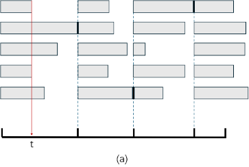
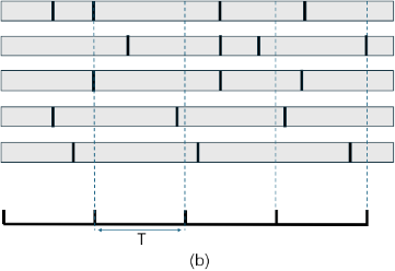
Figure 1. Asynchronous execution status in vectorized environment. (a. Agent updates synchronously despite asynchronous environment progress; b. Environments update independently, improving training efficiency.)
To control the error of return expectation, the algorithm integrates KL divergence restrictions with return estimation clipping. A hyperparameter threshold is set, where updates are performed only if the KL divergence remains within this threshold, otherwise, return estimates are clipped.
The author added three different regularization methods in the gradient update stage, which more cleverly balances the stability and generalization of the neural network than the traditional method.
Dominance function normalization: In the update stage, the small-batch dominance function is normalized
\( {A^{ \prime }}({s_{t}}, {a_{t}})= \frac{A({s_{t}}, {a_{t}})-E[A({s_{t}}, {a_{t}})]}{var[A({s_{t}}, {a_{t}})]} \) (1)
Gradient clipping: This paper limited the gradient to a pre-set threshold range c. If the L2 norm of the gradient is greater than this threshold, the L2 norm of the gradient is scaled to the threshold size without changing the direction of the gradient, which is formalized as follows
\( clip(∇f)=\begin{cases} \begin{array}{c} \frac{c∙∇f}{{‖∇f‖_{2}}},if {‖∇f‖_{2}} \gt c \\ ∇f,else \end{array} \end{cases} \) (2)
Entropy regularization loss: The uncertainty of a random variable can be measured by using the entropy regularization term. The author subtracted the entropy regularization term for the probability of each action strategy in a small lot from the loss function, as shown below.
\( {L_{entropy}}=\sum ^{batch}\sum _{ i=1}^{4}{P_{i}}\cdot log{{P_{i}}} \) (3)
By incorporating prior human knowledge into the model through reward mechanism adjustments, including life loss feedback and ineffective strategy punishment, the agent's scoring ability and anthropomorphic performance are improved.
To simplify the input state space, preprocessing steps include image resizing and grayscale conversion, reducing computational load and model training difficulty. Multi-frame stacking provides a comprehensive dynamic view of the environment, while a frame playback buffer maintains a queue to update frames continuously. Input normalization maps image pixel values to the [0, 1] interval, optimizing the network's learning process and ensuring training stability. Table 1 shows the value and remarks of hyperparameter.
Table 1. Value and remarks of hyperparameter.
TOTAL_TIMESTEPS | 50000000 | Total time steps for training |
LEARNING_RATE_1 | 2.5 e-4 | The segmented initial learning rate for the first half of the iteration |
LEARNING_RATE_2 | 1E-6 | The segmented initial learning rate for the second half of the iteration |
NUM_ENVS | 8 | Vectorized number of parallel environments |
NUM_STEPS | 128 | The number of sampling steps of data used in one iteration |
GAMMA | 0.99 | The exponential moving average coefficient used to calculate the return |
LAMBDA | 0.95 | Exponential moving average coefficient for the advantage function |
NUM_MINIBATCHES | 4 | The number of small batches (not the number of samples in small batches) |
UPDATE_EPOCHS | 4 | Number of updates |
CLIP | 0.1 | Return clipping (limiting the probability ratio to 1±CLIP) |
ENT_COEF | 0.01 | Entropy regular term coefficient |
VF_COEF | 0.5 | Value function mean square loss coefficient |
MAX_GRAD_NORM | 0.5 | Gradient clipping upper bound |
TARGET_KL | 0.12 | KL divergence upper bound |
2.3. Application of Machine Learning
2.3.1. Algorithm research and comparison. To facilitate the elaboration of the subsequent research results, the author let the Markov decision process be expressed as (S, A, P, R), where:
S: state space, representing the set of all possible states.
A: action space, which represents the set of all possible actions.
P: Transition probability function, representing the probability of moving to the next state s' given state s and action a, denoted as s, can also be expressed as, i.e \( P:S×A×S→[0,1]P(s,a,{s^{ \prime }})=p({s^{ \prime }}∣s,a) \) . The given | here is the conditional probability, i.e., the probability of s' given s and a.
R: reward function, which represents the reward obtained at a given state s, denoted R(s). \( R:S→R \)
This research compares the white box algorithm of interpretability algorithm (i.e., machine learning algorithm) for the purpose of the project, training an interpretable model based on the trained reinforcement learning model and the data generated by the interaction with the environment (breakout environment provided by OpenAI), and given a state, The output of this model can be consistent with the output of the reinforcement learning model, i.e[6][7]. :
\( π(s) = {π^{*}}(s) \) (4)
Where, is the strategy learned by the reinforcement learning model, is the strategy learned by the interpretable white box model, and s is the current state [1].
To achieve this, the author was faced with two questions, the first one is data acquisition.
To acquire the data, the model receives states as inputs and outputs actions during its interaction with the Breakout environment. In each iteration, all state-action (s-a) pairs are formed into a sub-dataset, and all sub-datasets together form the final dataset. This data is used to train the white-box model. Note that the state in the Breakout environment is actually an image and belongs to high-dimensional data, making it difficult to understand. Therefore, the author used computer vision technology to extract a state vector from each frame image, which includes the ball's motion direction on the X and Y axes, the ball's position (x, y coordinates), and the paddle's X coordinate:
\( {s^{*}}=({v_{x}},{v_{y}},{x,y,x_{p}})∈{S^{*}} \) (5)
i.e., there is a transition function:
\( t∶S→{S^{*}} \) (6)
With this feature extraction, the author got data pairs of the form, which provide the data needed to train the white-box model.
\( {S^{*}}×A \) (7)
Another one is model selection.
In the Breakout environment [8], the reinforcement learning model receives states as inputs and outputs one of four possible actions. This process can be viewed as a classification task. The author tested the performance of several classical interpretable classification models, various decision tree model variants, and several ensemble learning models. In terms of imitation learning methods, the author studied the effects of direct training and training with the Q-DAGGER [4] algorithm on training efficiency. In parameter adjustment, the author experimented with decision trees of different depths and different numbers of nodes.
The core of the gradient enhancement algorithm [9] is to use the negative gradient of the loss function to guide the learning of the model. Let's say our goal is to minimize the loss function \( (L(y,F(x))) \) , where the true value is the predicted value of the model \( (y) \) .In each iteration, the author wanted to add a new model \( (h(x)) \) that minimizes the loss function.
Initialize the model: The author started with an initial model, usually an average of the data or a constant that minimizes the loss function.
Iterative enhancement: In each iteration, the author calculated the negative gradient of the loss function, i.e., the residual:
(8)
Then, the author trained a new model to predict these residuals.
Update model: The author updated our model by adding a scaled new model:
(9)
Among them, \( (v) \) is the learning rate, which controls how much you update at each step.
Loss function optimization: By choosing \( {(h_{i}}(x)) \) to minimize the loss function, the author could ensure that each step moves in the direction of loss reduction.
Comparison of models trained based on Q-DAGGER simulation learning algorithm is shown in Table 2[4].
Table 2 shows the performance of the model trained based on Q-DAGGER simulation learning algorithm [4]. It can be seen from the table 2 that the gradient enhancement algorithm has the best performance, so the author chose it as the training algorithm for the final model.
Table 2. Model performance based on Q-DAGGER simulation learning algorithm training.
Model | CART decision tree | Random Forest | Gradient Enhancement |
Accuracy | 0.79 | 0.85 | 0.9 |
Recall rate | 0.79 | 0.85 | 0.88 |
F1-score | 0.79 | 0.86 | 0.89 |
Reward | 21.2 | 43.6 | 123.6 |
2.3.2. Experimental process. Seven key steps make up the experimental process: data collection, preprocessing, parameter setting, model training, model comparison, cross-validation, and performance evaluation.
Firstly, the author recorded the interactions between the PPO model and the game environment, specifically capturing state-action data pairs that collectively form our datasets. Secondly, this step involves performing the necessary preparations on the dataset. The author identified templates for each data pair and extracted the ball's horizontal and vertical coordinates, as well as the paddle's horizontal coordinates. In order to create a dataset of feature-action pairs, the author also calculated the ball's speed by analyzing its position before and after each data pair. Thirdly, for algorithms such as CART decision trees, random forests, and gradient boosting, the author adjusted key parameters, including the number of trees, depth, and learning rate, to determine the optimal configuration. Fourthly, using the prepared dataset, the author trained various models with different parameters to identify the one that performed best. Fifth, the author tests the best-performing model in the breakout environment to compare it to the baseline PPO model. Sixthly, the author used the K-fold cross-validation method to assess the stability and generalizability of the model. Finally, the author uses metrics like accuracy rate, recall rate, and F1 score to compare the model's performance to an oracle.
2.3.3. Parameter optimization and experimental comparison. The gradient enhancement model algorithm training based on Q-DAGGER simulation learning algorithm has achieved the best effect in all models, and in terms of parameter adjustment, it needs to be optimized [4]. Here is the cross-validation comparison of our experimental data:
|
|
Figure 2. Line chart of fit rate and average fit rate of the model based on 5000 decision tree 7 maximum tree depth. | Figure 3. Line graph of fit rate and average fit rate of model based on 0.01 learning rate 7 maximum tree depth |
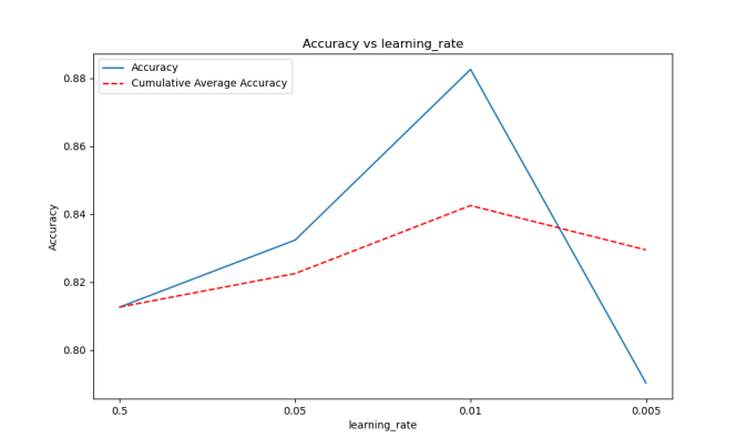
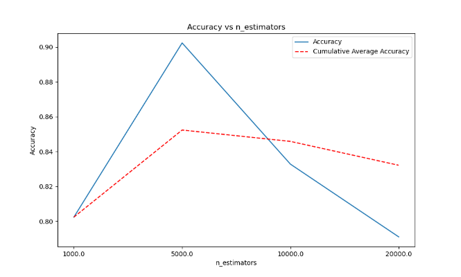
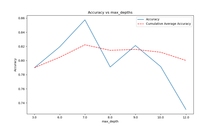
Figure 4. Line graph of fit rate and average fit rate of model based on 0.01 learning rate 5000 decision tree.
As shown in Figure 2, Figure 3, and Figure 4, the learning rate is 0.01, the maximum depth of the tree is 7, and the total number of decision trees is 5000. The trained model has the best performance; it is also the final model selected. We display the model's performance below:
|
|
Figure 5. Line chart of reward and average reward during 45 iterations of the model. | Figure 6. Line graph of fit rate and average fit rate during 45 rounds of model iteration. |
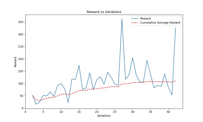
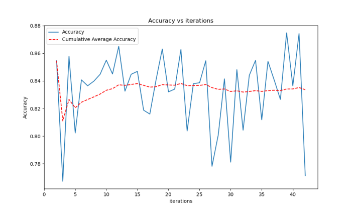
Figure 5 shows the reward and average reward during 45 iterations of the model. The reward curve demonstrates the model's learning progression, where an upward trend indicates improving performance as the model becomes more adept at maximizing rewards in the Breakout environment. The average reward curve smooths out the fluctuations, providing a clearer picture of the overall trend and confirming the model's learning stability over time. Figure 6 depicts the fit rate and average fit rate during 45 rounds of model iteration. The fit rate represents how well the model's actions match the optimal ones during training. A higher fit rate indicates better performance in terms of making correct decisions. The average fit rate provides a smoothed version of this metric, showcasing the model's improvement in decision-making accuracy as training progresses.
3. Analysis of Results
3.1. Reinforcement learning
|
|
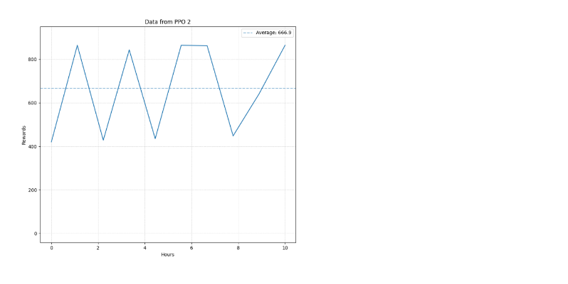
Figure 7. PPO Model 1 Score curve with training. | Figure 8. Model 1 is the score chart for each game in the test with an average score of 666.9. |
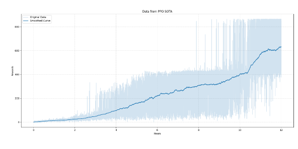
The abscissa is the training duration (hours), and the ordinate is the model's score in one game. The light color is the actual score data and the dark color is the smoothed score data.
|
|
Figure 9. Model 2 score curve with training. | Figure 10. Model 2 score chart for each game in the test with an average score of 499.7. |
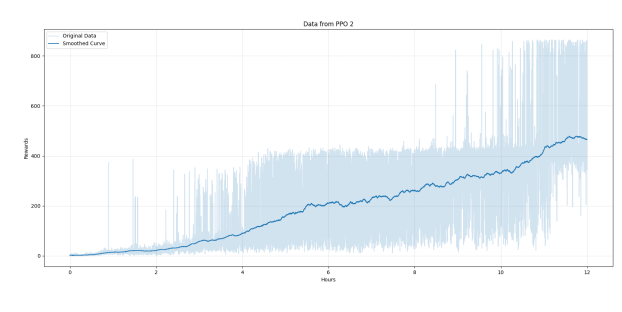

Figures 7, 8, 9, and 10 compare the performance of two different models, Model 1 (PPO) and Model 2 (an alternative model). Figures 7 and 8 focus on Model 1. Figure 7 shows the score curve with training, where the x-axis represents training duration in hours, and the y-axis represents the model's score in one game. The light color indicates actual score data, while the dark color shows smoothed data. The upward trend reflects Model 1's performance improvement over time. Figure 8 shows the score chart for each game in the test, with an average score of 666.9, indicating the PPO algorithm's consistent high performance and stability.
Figures 9 and 10 focus on Model 2. Figure 10 shows the training score curve, similar to Figure 7. Figure 9 shows the score curve with training, similar to Figure 7. The score curve for Model 2 shows slower improvement and more pronounced fluctuations, indicating less stability and efficiency compared to Model 1. Figure 10 presents the score chart for each game in the test, with an average score of 499.7, highlighting that Model 2, while moderately effective, does not achieve the same level of consistency and high scores as Model 1.
3.2. Interpretability algorithm
|
|
Figure 11. Line chart of reward change and average reward for ten rounds of games in the final model. | Figure 12. Line chart of fit rate change and average fit rate for ten rounds of final model games. |
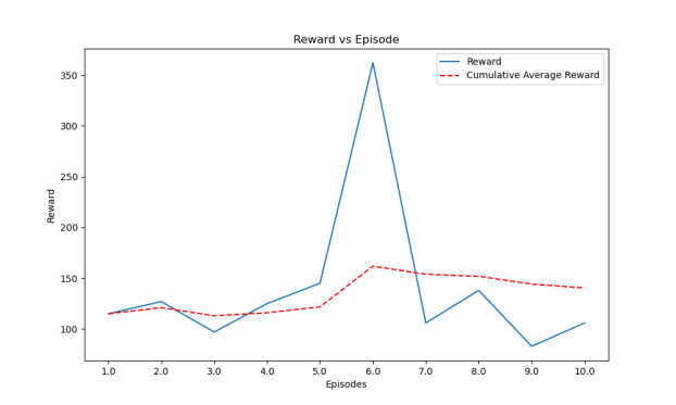
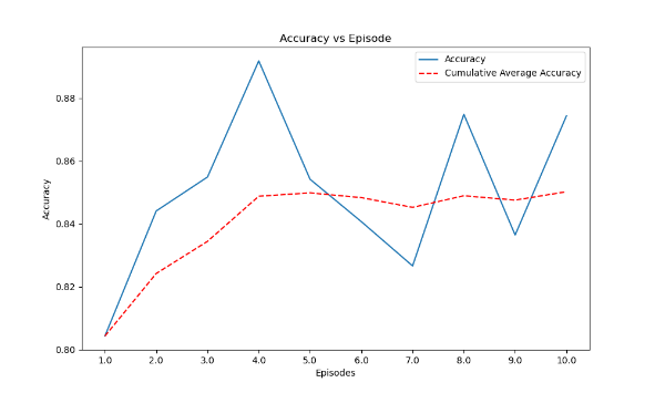
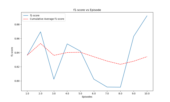
Figure 13. F1 score change and average F1 score line graph of the final model ten rounds game.
Figure 13 displays the F1 score change and the average F1 score line graph of the final model for the ten-round game.
The author ultimately chose the condensation simulation learning interpretability model from Figures 11, 12, and 13, using the Q-DAGGER [4] algorithm framework, and adopted a gradient-enhanced integrated learning algorithm based on a CART decision tree [7]. The parameters are set as follows: The parameters are set as follows: 5000 decision trees, a learning rate of 0.01, and a maximum depth of 7 for the decision tree. Ultimately, following multiple iterations and training learning, the model's final output reveals an average action fitting rate of 84%, an average F1 score of 0.84, and an average reward of 120 points resulting from the actual interaction with the breakout environment.
3.3. Interpretability analysis
('vector X for ball', 0.08479988978768412)
('vector Y for ball', 0.20390364198387242)
('coordinate X for ball', 0.26087393167295003)
('coordinate Y for ball', 0.2679382512176707)
('coordinate X for board', 0.1824828533782274)
It can be seen from above that the feature importance of the contribution of different environmental features to behavior prediction, among which the X vector features of the ball can best reflect the behaviors that affect the decision tree model, can lay a foundation for our preliminary understanding of the action of the decision tree [10].

Figure 14. The decision tree with the highest contribution from the final model.
Figure 14 illustrates the situation. The coordinate Y for the ball is less than 161.5. This is the decision rule for the node. It means that for the current node, if the value of the ball's ordinate is less than or equal to 137.0, the data will flow along the left branch; if it is greater than 137.0, it flows along the branch on the right.
friedman_mse = 0.03: This is the quality measure of the partition of this node. The Friedman mean square error (MSE) is a segmentation quality measure specific to gradient-enhanced models that takes into account the difference in mean values of the segmented child nodes and the sample weights. The value of 0.02 here represents the quality of the segmentation at that node and represents the difference in the target value of the segmented child nodes.
samples = 9: This indicates the total number of samples that were processed by that node. In this example, there are 9 samples of training data that satisfy the decision rule for the node.
The gradient-enhanced internal decision tree operates through a specific degree of regression task, resulting in a value of -0.67. This is because the model performs a weighted centralized output across all decision trees, ultimately achieving the target value through the computation of a weighted formula based on the learning rate. The value here represents the predicted value of the corresponding category of the current decision tree under this branch. Simultaneously, the author applied the aforementioned rules to each sub-node of 5000 decision trees, thereby determining the action probability of the decision tree under any environmental feature. This was achieved through complex calculations that took into account the influence of features on node segmentation, as well as the characteristics and sample flow of the corresponding nodes. This approach allowed for relatively accurate reasoning and generalization of the model's action logic.4
4. Conclusion
This project, which involved training a reinforcement learning agent in the OpenAI Gymnasium environment using algorithms such as PPO, Q-DAGGER, and gradient boosted decision trees, has produced significant results. The agent demonstrated robust performance improvements, especially with the PPO algorithm, showing a high score capability and a stable learning curve after extensive training and algorithmic refinement. The author also made strides in the interpretability of complex models by integrating machine learning techniques that mimic decision-making processes, which enhances the trustworthiness and understandability of the AI's decisions. However, the performance of our models heavily relies on the quality and diversity of the training data, suggesting that future research could benefit from exploring more diverse environments or multi-agent scenarios. Additionally, the computational demands of our project are substantial, and optimizing these algorithms for efficiency could be a focus for future iterations. Despite the progress in interpretability, we still need to make the decision-making processes of the models more transparent. Future studies could potentially explore novel visual or quantitative methods to further clarify AI decisions.
References
[1]. Reinforcement Learning Stability: Mnih, V., Kavukcuoglu, K., Silver, D., et al. (2015). Human-level control through deep reinforcement learning. Nature, 518(7540), 529-533.
[2]. Machine Learning for Decision Making: Ribeiro, M.T., Singh, S., & Guestrin, C. (2016). "Why should I trust you?": Explaining the predictions of any classifier. In Proceedings of the 22nd ACM SIGKDD international conference on knowledge discovery and data mining (pp. 1135-1144).
[3]. Proximal Policy Optimization (PPO): Schulman, J., Wolski, F., Dhariwal, P., Radford, A., & Klimov, O. (2017). Proximal policy optimization algorithms. arXiv preprint arXiv:1707.06347.
[4]. Q-DAGGER: Ross, S., & Bagnell, D. (2010). Efficient reductions for imitation learning. In Proceedings of the thirteenth international conference on artificial intelligence and statistics (pp. 661-668).
[5]. OpenAI Gymnasium: Brockman, G., Cheung, V., Pettersson, L., Schneider, J., Schulman, J., Tang, J., & Zaremba, W. (2016). OpenAI gym. arXiv preprint arXiv:1606.01540.
[6]. Reinforcement Learning Stability: Mnih, V., Kavukcuoglu, K., Silver, D., et al. (2015). Human-level control through deep reinforcement learning. Nature, 518(7540), 529-533.
[7]. Interpretable Machine Learning Models: Molnar, C. (2020). Interpretable machine learning. Lulu.com.
[8]. Machine Learning for Decision Making: Ribeiro, M.T., Singh, S., & Guestrin, C. (2016). "Why should I trust you?": Explaining the predictions of any classifier. In Proceedings of the 22nd ACM SIGKDD international conference on knowledge discovery and data mining (pp. 1135-1144).
[9]. Computational Demands in AI Research: Jordan, M.I., & Mitchell, T.M. (2015). Machine learning: Trends, perspectives, and prospects. Science, 349(6245), 255-260.
[10]. Visual Methods for Model Interpretability: Zeiler, M.D., & Fergus, R. (2014). Visualizing and understanding convolutional networks. In European conference on computer vision (pp. 818-833).
Cite this article
Chen,Y. (2024). Enhancing stability and explainability in reinforcement learning with machine learning. Applied and Computational Engineering,101,25-34.
Data availability
The datasets used and/or analyzed during the current study will be available from the authors upon reasonable request.
Disclaimer/Publisher's Note
The statements, opinions and data contained in all publications are solely those of the individual author(s) and contributor(s) and not of EWA Publishing and/or the editor(s). EWA Publishing and/or the editor(s) disclaim responsibility for any injury to people or property resulting from any ideas, methods, instructions or products referred to in the content.
About volume
Volume title: Proceedings of the 2nd International Conference on Machine Learning and Automation
© 2024 by the author(s). Licensee EWA Publishing, Oxford, UK. This article is an open access article distributed under the terms and
conditions of the Creative Commons Attribution (CC BY) license. Authors who
publish this series agree to the following terms:
1. Authors retain copyright and grant the series right of first publication with the work simultaneously licensed under a Creative Commons
Attribution License that allows others to share the work with an acknowledgment of the work's authorship and initial publication in this
series.
2. Authors are able to enter into separate, additional contractual arrangements for the non-exclusive distribution of the series's published
version of the work (e.g., post it to an institutional repository or publish it in a book), with an acknowledgment of its initial
publication in this series.
3. Authors are permitted and encouraged to post their work online (e.g., in institutional repositories or on their website) prior to and
during the submission process, as it can lead to productive exchanges, as well as earlier and greater citation of published work (See
Open access policy for details).
References
[1]. Reinforcement Learning Stability: Mnih, V., Kavukcuoglu, K., Silver, D., et al. (2015). Human-level control through deep reinforcement learning. Nature, 518(7540), 529-533.
[2]. Machine Learning for Decision Making: Ribeiro, M.T., Singh, S., & Guestrin, C. (2016). "Why should I trust you?": Explaining the predictions of any classifier. In Proceedings of the 22nd ACM SIGKDD international conference on knowledge discovery and data mining (pp. 1135-1144).
[3]. Proximal Policy Optimization (PPO): Schulman, J., Wolski, F., Dhariwal, P., Radford, A., & Klimov, O. (2017). Proximal policy optimization algorithms. arXiv preprint arXiv:1707.06347.
[4]. Q-DAGGER: Ross, S., & Bagnell, D. (2010). Efficient reductions for imitation learning. In Proceedings of the thirteenth international conference on artificial intelligence and statistics (pp. 661-668).
[5]. OpenAI Gymnasium: Brockman, G., Cheung, V., Pettersson, L., Schneider, J., Schulman, J., Tang, J., & Zaremba, W. (2016). OpenAI gym. arXiv preprint arXiv:1606.01540.
[6]. Reinforcement Learning Stability: Mnih, V., Kavukcuoglu, K., Silver, D., et al. (2015). Human-level control through deep reinforcement learning. Nature, 518(7540), 529-533.
[7]. Interpretable Machine Learning Models: Molnar, C. (2020). Interpretable machine learning. Lulu.com.
[8]. Machine Learning for Decision Making: Ribeiro, M.T., Singh, S., & Guestrin, C. (2016). "Why should I trust you?": Explaining the predictions of any classifier. In Proceedings of the 22nd ACM SIGKDD international conference on knowledge discovery and data mining (pp. 1135-1144).
[9]. Computational Demands in AI Research: Jordan, M.I., & Mitchell, T.M. (2015). Machine learning: Trends, perspectives, and prospects. Science, 349(6245), 255-260.
[10]. Visual Methods for Model Interpretability: Zeiler, M.D., & Fergus, R. (2014). Visualizing and understanding convolutional networks. In European conference on computer vision (pp. 818-833).