1. Introduction

The emergence of the Kolmogorov-Arnold Network (KAN) proposed by Liu et al. has led to a new direction in the existing research on neural network architectures [1]. It changes the complex structure in the traditional multilayer perceptron (MLP) by moving the training objects from the individual nodes in the neural network to the edges, i.e., the individual spline functions [2]. This not only greatly improves the efficiency of the neural network, but also simplifies the network structure, allowing KAN to use a smaller scale number of parameters for deep learning tasks. It has also enabled the updating of many applications in the field of deep learning, such as the replacement of the MLP layer in convolutional neural networks (CNNs) in Cheon's research on KAN convolution, which has led to better performance with KAN than with MLP for small datasets with the same parameter scales [3].

Cheon mentions in the paper that their research has some limitations, they only utilized a small-scale dataset to complete the experimental exploration, but the performance of KAN for a certain task in a detailed domain is not yet known [3]. Therefore, in this paper, author will explore the performance of MLP structure using KAN structure instead of Feed-forward Neural Network (FFN) in Vision Transformer (ViT) in the field of lung ultrasound in computer vision medicine [4,5].

In the field of medical ultrasound, the scoring mechanism of the lungs (usually a score of 0-3) is primarily used to assess a patient's lung health status, especially in the diagnosis and monitoring of diseases such as Acute Respiratory Distress Syndrome (ARDS) or pneumonia [6]. This scoring system, commonly referred to as the Lung Ultrasound Score (LUS), is used to quantitatively assess the degree of lung involvement. In LUS, doctors classify the condition on a scale of 0-3 based on the patient's lung ultrasound images, and as the score increases, it means that the patient's condition is more severe. LUS has immeasurable value in clinical adjuvant therapy because it is non-invasive and it can be used in both high- and low-resource settings [7]. LUS is a composite score based on the A-lines, B-lines, shape of pleural line, and areas of consolidation on the patient's ultrasound image [7]. Thus, the scoring of a condition can be viewed as a classification task in computer vision.

In this paper, the author will try to construct a ViT model using KAN, use it as an aid in the diagnosis of clinical images of lung ultrasound, and prove its better performance by comparing the experimental results obtained with the traditional MLP implementation of the ViT model.

2. Method

2.1. Kolmogorov-Arnold Networks

The theoretical foundation of KAN comes from Kolmogorov-Arnold theory, the core idea of which is that any n-dimensional multivariate continuous complex function can be represented by a linear combination of several simple one-dimensional continuous functions, and KAN inherits this idea. Compared to the traditional MLP structure that uses fixed activation functions, e.g., Rectified Linear Unit (ReLU) and Sigmoid, on nodes, a.k.a. neurons, KAN moves the trainable spline activation functions to individual edges, a.k.a. weights, making the individual spline functions parameterized [1]. This allows approximating a complex function \( f(x) \) by linear combinations and transformations between individual spline parameterized functions \( \varphi_{q,p} \) . The Kolmogorov-Arnold theory can be expressed as:

\( f\left(x\right)=\sum_{q=1}^{2n+1}{\mathrm{\Phi}_q(\sum_{p=1}^{n}{\varphi_{q,p}(x_p)})} \) (1)

, where \( x_p \) is an input feature, \( \varphi_{q,p} \) is a parameterized activation function (spline function) and \( \mathrm{\Phi}_q \) is a linear combination of activation functions.

In KAN, B-spline functions are used as activation functions. These spline functions are segmented polynomials, defined by control points and knots. The B-spline function is particularly suitable for use as an activation function \( \varphi_{q,p} \) in KAN because of its flexibility in fitting complex nonlinear relationships, which can be expressed as:

\( \varphi\left(x\right)=w(b\left(x\right)+spline(x)) \) (2)

, where \( w \) is a weight and \( b\left(x\right) \) is a basis function, realized here by the Sigmoid Linear Unit (SiLU) with the mathematical expression is:

\( b\left(x\right)=SiLU\left(x\right)=\frac{x}{1+e^{−x}} \) (3)

And \( spline(x) \) is the spline function which can be expressed as:

\( spline\left(x\right)=\sum_{i}{c_iB_i(x)} \) (4)

, where \( c_i \) is the coefficients obtained by training learning. And \( B_i(x) \) is the B-spline base function, which is a segmented polynomial used to generate more complex curves or functions. These basis functions are used to construct spline curves for more complex patterns or data distributions. As stated by Liu et al: Compared to the complex structure of MLP, KAN has more interpretability as well as better performance, making it an effective alternative to MLP [1].

2.2. Vision Transformer

The core theory of ViT stems from Transformer, which has revolutionized the field of NLP. And in the field of computer vision, the limitations of ViT's dependence on CNNs have been addressed by Dosovitskiy et al., allowing it to achieve equally good performance in this area [5]. The core idea of ViT is to segment an image into multiple fixed-size patches and then spread these patches into a one-dimensional sequence. Unlike traditional CNNs, ViT relies entirely on Self-Attention Mechanism (SAM) to process image data [8,9]. Compared to the layer-by-layer extraction of features through local receptive fields in CNNs, ViT enables the model to capture global dependencies by representing the entire image as a sequence [5].

2.3. KAN+ViT

As mentioned above, the MLP structure is still used in ViT, therefore, this work tries to use the KAN structure in ViT instead of the original MLP to try to improve its performance.

Input. The input \( X \) to the model is a tensor of the shape \( [B,C,H,W] \) , denoting the batch size, number of channels, height and width respectively. The input image will be converted into this type of data and handed over to the model for processing.

Patch embedding. First, the size of the patch is set and then the input image is transformed into the form of fixed size patches. Assuming that the size of each patch is \( [P,P] \) , the height \( H \) and width \( W \) of the image must be a multiple of \( P \) so that the image can be completely divided into \( (\frac{H}{P})\times(\frac{W}{P}) \) patches. Then for each block, it needs to be flattened into a one-dimensional vector. Assuming that the image has \( C \) channels (e.g. an RGB image has 3 channels), then the length of the vector after flattening is \( P\times P\times C \) for each block. The image is re-formed into a set of patches, denoted \( X_{patch} \) , of shape is:

\( X_{patches}=reshape(X,[B,N,P^2\bullet C]) \) (5)

, where \( B \) is the batch size, i.e., the number of images per input; \( N \) is the number of patches, i.e., \( (\frac{H}{P})\times(\frac{W}{P}) \) ; \( P^2 \) is the number of pixels in each block after spreading, and \( P^2 \) is the number of pixels within the patch to be multiplied by the number of channels \( C \) .

This operation can be realized by a 2D convolutional layer, which is used to divide the input image into non-overlapping patches and map these patches into a \( D \) -dimensional embedding representation. The size of the convolution kernel should be equal to the size of the patch, and the step size should be set to the size of the patch, so that each patch is processed individually and there is no overlap:

\( X^\prime=W\ast X+b \) (6)

, where \( W \) is the convolutional kernel, \( X \) is the input image, \( b \) is the bias, and \( X_{patches} \) denotes the result of the image being divided into patches, each of which is mapped into an \( D \) -dimensional embedding space.

2.3.3. Position embedding and classification token. Before entering the ViT encoder, it is also necessary to add the position embedding and classification token, which are used to represent the positional information of the image and the classification information of the image, respectively. The classification token is a learnable vector that represents the global information of the entire image and is added in front of all block embeddings:

\( X_{CLS}=[CLS|X^\prime] \) (7)

It is shaped as:

\( X_{{patches}^\prime}=[B,N+1,D] \) (8)

, where \( N+1 \) denotes the number of patches after adding the Classification Token, and \( D \) is the size of the spatial dimension of each patch embedding (determined by the model itself). And the positional encoding is a learnable vector \( PE \) that adds positional information to each block, enabling the model to perceive the relative position of each block in the original image:

\( X_{POS}=X_{CLS}+PE \) (9)

\( X_{POS} \) is the input to which the position vector has been added, after which it can be entered into the ViT Encoder.

2.3.4. ViT encoder. The ViT Encoder consists of multiple Transformer encoder layers stacked together, each layer is divided into two parts: a multi-head attention mechanism and a feed-forward neural network, and its structure is referenced to Alexey et al.'s study [5]. The architecture is demonstrated in Figure 1.

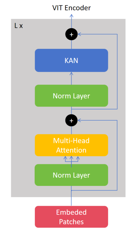
Figure 1. Architecture of ViT encoder (Figure Credits: Original).

The encoder processes the input sequence in several steps. First is layer normalization, where the input embedded sequence is first normalized by layers to normalize and stabilize the subsequent attention computation:

\( X_{norm}=LayerNorm(X_{pos}) \) (10)

The model then computes the attentional weights for each position in the input sequence through a multi-head self-attention (MHSA) mechanism and updates the representation of each position:

\( X_{attn}=MHSA(X_{norm}) \) (11)

It is then added back to the original input via the residual connection:

\( X^\prime=X_{pos}+DropPath(X_{attn}) \) (12)

The updated representation is later passed through a KAN (replacing the original MLP here) to further extract features. Similarly, the output of the KAN is added back to the input via a residual connection:

\( X_{out}=X^\prime+DropPath(KAN(X^\prime)) \) (13)

The above operation is repeated for each layer of the encoder. After stacking multiple layers of encoder, the final output contains global features that will be used for downstream classification tasks. And in the last layer of the encoder, KAN will extract the classification markers that contain global information about the whole image and use them for the final classification task:

\( {CLS}_{out}=X_{out}[:,0,:] \) (14)

Output. Ultimately, the output \( {CLS}_{out} \) is fed into a classifier header which maps the final predicted classification result to a probability distribution by fitting a Softmax function via KAN:

\( logits=ClassifierHead({CLS}_{out}) \) (15)

\( P\left(y=c\middle| l o g i t s\right)=\frac{e^{{logits}_c}}{\sum_{c^\prime} e^{{logits}_{c^\prime}}} \) (16)

\( \hat{y}={argmax}_cP(y=c|logits) \) (17)

, where \( c \) is the class label, \( P\left(y=c\middle| l o g i t s\right) \) is the probability that the image belongs to class \( c \) , and \( \hat{y} \) is the final output of the model.

3. Experiment and Result

3.1. Dataset

The dataset used in this paper was provided by the Emergency Department of Changzheng Hospital, Shanghai, China, in which all images were derived from patients with clinical pneumonia, including ultrasound videos of patients at several different periods, e.g., during the period of neocoronary pneumonia. Representative examples are demonstrated in Figure 2. And keyframe extraction and dataset filtering were performed by the authors of this paper and integrated. This dataset ensures clinical authenticity, maximizes the reproduction of data sampled in real clinics, and enables the most realistic testing of model performance. However, it is worth noting that the amount of data available for training is limited because of the privacy and limitations of the data (some frames do not respond properly to LUS), so the results derived from this experiment may also be partially affected, but it is not a hindrance to the judgment of the results. In this experiment, the training set has a total of 2846 samples and the validation set has a total of 567 samples, which are divided according to the ratio of 1:5, and there are 4 classes (0-4 points).

3.2. Experimental settings

The first experiment is used to test the performance of the two models on the lung ultrasound dataset. In this experiment, there are five main hyperparameters to focus on. The first is the number of epochs, due to the large number of parameters in ViT itself and the large amount of GPU memory it takes up, in this experiment the epoch is set to 200, which means that the model needs to traverse the dataset a total of 200 times. Since medical image data is limited, epoch does not need to be set a lot to compare the performance gap between KAN+ViT and ViT from the training results. Second is the batch size, in this experiment, the batch size is set to 32, which means that there are 32 dataset samples in each batch, and these 32 samples are processed in parallel and used to compute the gradient update of the model. Since the training set has 2846 samples and batch size 32, there should be 89 batches in each epoch. The models used are ViT and ViT with MLP replaced by KAN (ViT+KAN), respectively. Then, there is learning rate. In this experiment the authors set two learning rates, initial learning rate 0.0002 and final learning rate 0.0001, and used Cosine Annealing algorithm to adjust the learning rate dynamically [1]. Doing so makes the learning rate decrease as a cosine curve during training. The goal is to keep the model's learning rate high in the early stages of training to allow for rapid convergence; And the learning rate is gradually reduced at a later stage so that the model can converge more stably to a locally optimal solution. Finally, it is worth noting that since the visual model used for ultrasound imaging is quite specific, in order to ensure the accuracy of the experimental results, the authors did not use pre-trained weights for transfer learning in this experiment.

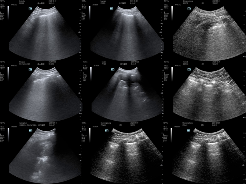
Figure 2. Representative examples of the ultrasound clinical imaging of the lungs (Figure Credits: Original).

In another experiment, the authors attempted to conduct a performance comparison test on the Cifar-10 dataset to compare the performance difference between MLP+ViT and KAN+ViT [10]. In this experiment, epoch was set to 50 and the rest of the parameters were consistent with the 3.2.1 experiment. The purpose of this experiment is in order to demonstrate that KAN+ViT still has better performance than ViT when using other types of datasets, and therefore does not require too many epoch numbers.

3.3. Evaluation criteria

Both of the above experiments in this paper use two dimensions as the evaluation criteria for the model performance: the first one is the change of loss in training; the second one is the change of accuracy in the validation set. Combining these two dimensions, a comprehensive evaluation of the model performance can be made.

3.4. Performance comparison

Ultrasound clinical imaging of the lungs. As shown in Figure 3, the KAN+ViT model exhibits a significant advantage in terms of training loss (blue curve). The training loss of the KAN+ViT model decreases rapidly at the beginning of training, and shows a stable decreasing trend throughout the training process. And with the increase of epoch, the curve decreases at a significantly higher rate than that of MLP+ViT, and finally reaches a lower loss level at the end of training ( \( \approx \) 0.326). This suggests that the KAN+ViT model has a strong learning capability and is able to fit the training data effectively. In contrast, the MLP+ViT model (yellow curve) has a smoother decline in training loss in the later stages, and although it also continues to decline with the training process, the overall loss level is higher than that of the former ( \( \approx \) 0.384).

The comparison of validation accuracies further highlights the difference in generalization ability between the two models. The accuracy of the KAN+ViT model on the validation set rises rapidly at the beginning of training and reaches a high level close to 0.9 after about 100 epochs, and remains stable with small fluctuations in the subsequent training process, finally reaching 0.981. In contrast, the validation accuracy of the MLP+ViT model rises at almost the same rate in the early stage, but the growth rate tends to decrease with the increase of epochs. The rate of increase tends to decrease, and the accuracy rate finally reaches only the level of 0.951.

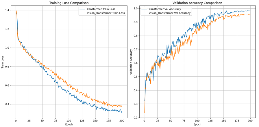
Figure 3. Model performance in lung ultrasound dataset (Figure Credits: Original).

In summary, compared with the traditional MLP+ViT model, the KAN+ViT model performs better in both training loss and validation accuracy, showing stronger learning ability and generalization ability, indicating that KAN+ViT performs better in lung ultrasound image classification compared with the traditional MLP+ViT.

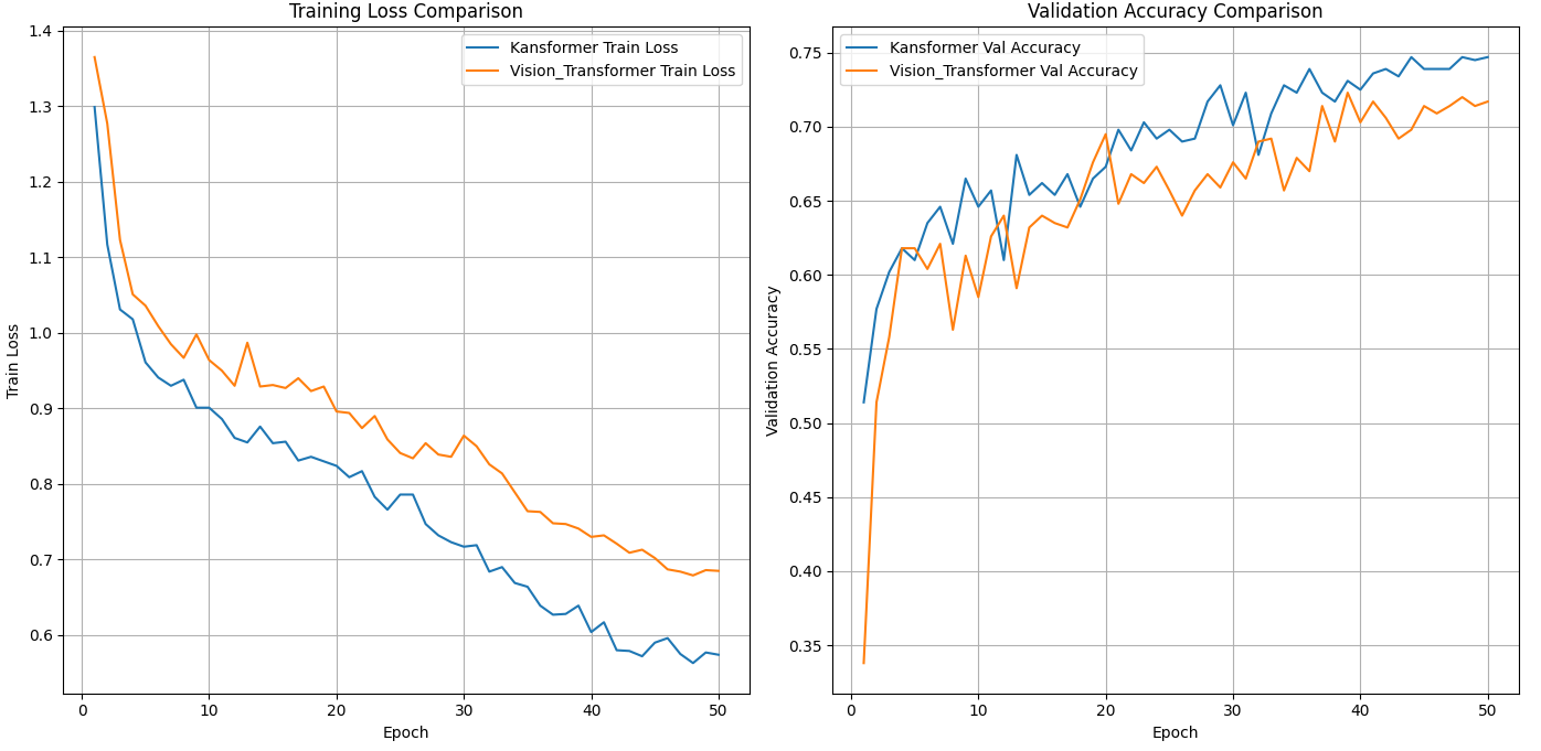
Figure 4. Model performance in Cifar-10 dataset (Figure Credits: Original).

Cifar-10. As shown in Figure 4, in this experiment, the authors compare the performance of two models, KAN+ViT and MLP+ViT, on the Cifar-10 training set and validation set. From the comparison of training loss, the training loss of KAN+ViT decreases significantly faster than that of MLP+ViT and shows a more stable decreasing trend throughout the training process, eventually reaching a lower training loss (<0.6). This suggests that KAN+ViT has a better fit on the training data and is able to learn the feature patterns in the data better. In contrast, the training loss of MLP+ViT decreases slightly slower and reaches a final loss between 0.6 and 0.7, which is clearly greater than that of KAN+ViT. In the comparison of validation set accuracies, the accuracy of the KAN+ViT model rises rapidly in the early stages of training and reaches a high and more stable level ( \( \approx \) 0.75) in the later stages of training; However, the validation set accuracy of MLP+ViT, while rising more slowly and eventually reaching a similar level to the KAN+ViT model, achieves significantly lower accuracy than the former.

Overall, KAN+ViT outperforms MLP+ViT in terms of fitting on the Cifar-10 training set, while the accuracy on the validation set remains high, showing a good balance, as demonstrated in Table 1. Combined with Experiment 3.4.1, it can be demonstrated that KAN+ViT generally possesses better performance than traditional MLP+ViT.

Table 1. Comparison of models on CIFAR-10, and lung clinical imaging datasets.

4. Conclusion

In summary, this paper realizes a new network architecture of KAN+ViT by replacing the MLP part of the traditional ViT with the higher performance KAN, and completes the exploration of the performance of this new network architecture and the performance comparison with the traditional MLP+ViT by designing experiments on different datasets. In this paper, KAN+ViT presents better performance compared to MLP+ViT on lung clinical ultrasound dataset and Cifar-10 respectively. Thus this study demonstrates the excellent promise of utilizing KAN+ViT in the field of visually assisted clinical diagnosis and the potential of the new architecture (KAN+ViT) over the traditional ViT architecture.

References

[1]. Liu, Z., Wang, Y., Vaidya, S., Ruehle, F., Halverson, J., Soljačić, M., ... & Tegmark, M. (2024). Kan: Kolmogorov-arnold networks. arXiv preprint arXiv:2404.19756.
[2]. Gardner, M. W., & Dorling, S. R. (1998). Artificial neural networks (the multilayer perceptron)—a review of applications in the atmospheric sciences. Atmospheric environment, 32(14-15), 2627-2636.
[3]. Cheon, M. (2024). Demonstrating the efficacy of kolmogorov-arnold networks in vision tasks. arXiv preprint arXiv:2406.14916.
[4]. Han, K., Wang, Y., Chen, H., Chen, X., Guo, J., Liu, Z., ... & Tao, D. (2022). A survey on vision transformer. IEEE transactions on pattern analysis and machine intelligence, 45(1), 87-110.
[5]. Dosovitskiy, A., Beyer, L., Kolesnikov, A., Weissenborn, D., Zhai, X., Unterthiner, T., ... & Houlsby, N. (2020). An image is worth 16x16 words: Transformers for image recognition at scale. arXiv preprint arXiv:2010.11929.
[6]. Ma, H., Yan, W., & Liu, J. (2020). Diagnostic value of lung ultrasound for neonatal respiratory distress syndrome: a meta-analysis and systematic review. Medical ultrasonography, 22(3), 325-333.
[7]. Smit, M. R., Mayo, P. H., & Mongodi, S. (2024). Lung ultrasound for diagnosis and management of ARDS. Intensive care medicine, 1-3.
[8]. Niu, Z., Zhong, G., & Yu, H. (2021). A review on the attention mechanism of deep learning. Neurocomputing, 452, 48-62.
[9]. Li, Z., Liu, F., Yang, W., Peng, S., & Zhou, J. (2021). A survey of convolutional neural networks: analysis, applications, and prospects. IEEE transactions on neural networks and learning systems, 33(12), 6999-7019.
[10]. Cifar-10 Dataset. URL: https://www.cs.toronto.edu/~kriz/cifar.html. Last Accessed: 2024/08/27.
Cite this article
Li,Z. (2024). A comparative study of KAN transformer and traditional vision transformer for ultrasound image-based diagnosis. Applied and Computational Engineering,103,109-116.
Data availability
The datasets used and/or analyzed during the current study will be available from the authors upon reasonable request.
Disclaimer/Publisher's Note
The statements, opinions and data contained in all publications are solely those of the individual author(s) and contributor(s) and not of EWA Publishing and/or the editor(s). EWA Publishing and/or the editor(s) disclaim responsibility for any injury to people or property resulting from any ideas, methods, instructions or products referred to in the content.
About volume
Volume title: Proceedings of the 2nd International Conference on Machine Learning and Automation
© 2024 by the author(s). Licensee EWA Publishing, Oxford, UK. This article is an open access article distributed under the terms and
conditions of the Creative Commons Attribution (CC BY) license. Authors who
publish this series agree to the following terms:
1. Authors retain copyright and grant the series right of first publication with the work simultaneously licensed under a Creative Commons
Attribution License that allows others to share the work with an acknowledgment of the work's authorship and initial publication in this
series.
2. Authors are able to enter into separate, additional contractual arrangements for the non-exclusive distribution of the series's published
version of the work (e.g., post it to an institutional repository or publish it in a book), with an acknowledgment of its initial
publication in this series.
3. Authors are permitted and encouraged to post their work online (e.g., in institutional repositories or on their website) prior to and
during the submission process, as it can lead to productive exchanges, as well as earlier and greater citation of published work (See
Open access policy for details).