1. Introduction

Multi-Agent Reinforcement Learning (MARL) has emerged as a critical subfield within the broader domain of Deep Reinforcement Learning (DRL), playing a pivotal role in the development and deployment of intelligent systems in complex, dynamic environments. Compared to the classical reinforcement learning methods that mainly focus on maximizing the rewards to select potential best policy for a single agent, MARL not only requires to make real-time decisions in response to a rapidly changing environment but also to engage in intricate interactions with other agents, showing a promising result in promoting various large-scale applications, such as robot collaboration, e-sports.

Existing MARL approaches mainly follow a two-stage framework, where each agent learns the interaction with the environment and then communicate through some well-designed strategies. As a cornerstone of the deep reinforcement learning, Deep Q-Network (DQN) integrates the classic Q-learning with deep neural networks for the first time [1], which leverages the powerful non-linear transformation ability of the convolutional neural network to alleviate the generalization challenges faced by Q-learning in high-dimensional state spaces. The success of DQN attracts increasing attention from both academic and industry, and researchers further explore its potential applications in multi-agent environments. One of the representative solutions is directly applying DQN to Independent Q-Learning, where each agent operates its own DQN instance and treats the actions of other agents as part of the environment [2]. However, because the strategies of agents in multi-agent systems dynamically influence the environment, Independent Q-Learning (IQL) encountered issues of instability and poor convergence during the learning process. To address these challenges, researchers proposed the Centralized Training, Decentralized Execution (CTDE) framework [3][4]. CTDE enhances the stability and efficiency of policy learning by allowing agents to share information during the centralized training phase, enabling joint optimization within a global environment model. During the execution phase, each agent acts independently based on the strategies learned during training. Inspired by the CTDE framework, Rashid et al. [3] combine different individual agents' Q-value functions based on a hybrid network architecture, which contributes to more flexibly Q-values optimized under the constraints of a global Q-value function. Sunehag et al. [4] propose the Value-Decomposition Networks (VDN), which approximates the global Q-value function by linearly combining the Q-values of individual agents. Though these methods have achieved significant progress, we argue their adaptability and performance are still affected by two serious issues. Firstly, the past structure in MARL always suffered from the issue of Q-value overestimation [5] and the inability to effectively distinguish between state values and action advantages [6]. Secondly, during the training stage, the traditional model inefficiently allocate computational resources, especially wasting computing sources on low-quality epochs [7], thus frequently ignored high TD errors which were critical for preserving the total efficiency and refining the model's accuracy.

To address the core challenges encountered, we propose an adaptive Multi-layer Attention Double Dueling Deep Q-Network (MAD-D3QN) for the multi-Agent reinforcement learning. Specifically, we first develop a two-layer attention module to dynamically adjust the computation of Q-values. The first attention layer calculates initial weights from feature vectors extracted from fully connected and convolutional layers, which will be used to generate intermediate weights by balancing the value and advantage components. The second layer further refines these intermediate weights and integrates them into the dueling DQN Q-value computation formula. To encourage a deeper collaboration among different agents, we introduce a weight allocation mechanism based on the trajectory quality of each deduction. By assigning higher update weight for the agent with high-TD trajectory, we accumulate the reward of each agent in a dynamic manner by considering the reward of their own and other agents, which helps optimize the whole model for a global best performance and improve computational efficiency during training. Extensive experiments are conduct to demonstrate the effectiveness of our method, involving the combinations of maps, difficulty levels, and agent quantity using the StarCraft II environment. To summarize, our main contributions include:

(1) This paper proposes a novel adaptive attention-based deep Q-Network, as the first attempt to combine the Double DQN and Dueling DQN in the MARL task.

(2) This paper develops a weight allocation mechanism based on the trajectory quality, which boosts more complementary collaboration among agents and significantly accelerate the training speed.

(3) This paper evaluates the proposed method through extensive experiments, outperform the previous methods by a large margin in various settings.

2. Related Work

2.1. D3QN Methodologies

The development of Multi-Agent Reinforcement Learning (MARL) benefits from the traditional Q-learning algorithm and its evolutions, such as Deep Q-Networks (DQN). Q-learning algorithm calculates the expected return for choosing a particular action in a specific state by learning the action-value function \( Q(s,a) \) [8]. By using neural networks to approximate the Q-value function, DQN avoids the direct storage of huge Q-value tables [1], thus extending the application of Q-learning to a high-dimensional state space. The Independent DQN (IDQN) adapts the DQN to the multi-agent environment [2], where each agent learns its own DQN model from interactions within the environment to make decisions. Further extensions like Double DQN [5] and Dueling DQN [6] have found significant applications in MARL. The MAD3QN model (Dueling Double DQN) integrates the strengths of Double DQN and Dueling DQN, which offers a more robust and efficient framework for tackling the complexities of multi-agent environments. By combining the double network structure of DDQN, D3QN mitigates overestimation bias in Q-value estimation by using two separate networks for action selection and target Q-value calculation. Meanwhile, beneficial from the dueling Q function, MAD-D3QN decomposes the Q-value into state value and action advantage. All the combinations improve the stability and convergence of strategies by enabling faster identification of effective policies in MARL environments, providing more accurate Q-value estimates and policy search.

2.2. CTDE Structure

Centralized Training with Decentralized Execution (CTDE) is a key paradigm in MARL that addresses challenges like instability and coordination difficulties. In detail, CTDE optimizes strategies using global information during training, while agents act independently based on local observations during execution. Also, the core advancements include VDN [9], which decomposes global Q-values into the sum of individual agents' Q-values, allowing for straightforward coordination through additive value functions. QMIX uses a nonlinear mixing network to combine individual Q-values conditioned on the global state, enables the modeling of complex inter-agent interactions[8]. Furthermore, COMA and MADDPG enhance policy gradients with centralized critics, introducing a centralized critic that computes advantage functions for each agent, conditioned on the joint actions of all agents, to improve credit assignment in cooperative settings. [10-11].

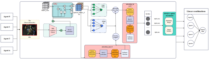
Figure 1. The pipeline of our proposed MAD-D3QN network. MAD-D3QN processes observations through layers, GRU, attention mechanisms, and DDQN updates, computing and combining Q-values across agents to optimize learning in multi-agent environments.

3. Methodology

3.1. Overview

The framework of our MAD-D3QN is shown in Figure 1. Each agent obtains observations from the environment, which is processed through a fully connected layer followed by a ReLU activation function. The output, along with the hidden state, is fed into a Gated Recurrent Unit (GRU) to capture temporal dependencies and update the hidden state over time. Taking all all the former outputs as input, a two-layer attention module sharing similar internal structure are introduced to calculate the weight parameters. Subsequently, the model calculates the state value and advantage functions, which respectively represent the intrinsic value of the current state and the relative advantage of different actions, equipping with the calculated weigh parameters. After obtaining Q-value and making relative action-decisions, the Double DQN (DDQN) update mechanism is employed to mitigate overestimation bias in Q-value estimation. Finally, based on the VDN model, the Q-values from multiple agents are linearly combined to form total Q-value and facilitate cooperative strategy learning.

3.2. Multi-layered Attention Dynamic D3QN Module

Each agent identifies the state and obtains the observation \( {O_{t}} \) , containing the shape of each agent's observation space, action information for the previous time step and the agent numbers. Afterwards, we utilize a fully connected layer to map the observation to a high-dimensional space to obtain eigenvectors. In the following stage, we input the eigenvector into the GRU unit to get the hidden state at the current moment, regarded as \( {h_{t}} \) . The first-level attention mechanism calculates the preliminary dynamic weight \( {α_{1}} \) and \( {β_{1}} \) according to the hidden state \( {h_{t}} \) . On the second-level attention mechanism, the combined weights are further adjusted to generate the final dynamic weights \( {α_{2}} \) and \( {β_{2}} \) :

\( \begin{cases}\end{cases}\ \ \ (1) \)

where \( {W_{1}} \) and \( {W_{2}} \) are the intermediate results obtained through these linear transformations and the ReLU activation function, which are then passed through the Softmax function to generate attention weights \( {α_{1}} \) , \( {β_{1}} \) and \( {α_{2}} \) , \( {β_{2}} \) . \( {α_{1}} \) and \( {β_{2}} \) adjust the first combination of the state value V(s) and the advantage function A(s, a), while \( {α_{2}} \) and \( {β_{2}} \) further refine these values to produce the final Q-value. W4 and W5 are weight matrices in the neural network that apply linear transformations to the input hidden state and intermediate results, helping adjust the output of the network layers. b4 and b5 are bias vectors added to the results of these linear transformations to further refine the output. With the two weights obtained through equation (1), the Q value of Dueling DQN is updated as:

\( Q({s_{t}},{a_{t}})={α_{2}}V({s_{t}},{a_{t}})+{β_{2}}(A({s_{t}},{a_{t}})-\frac{1}{|A|}∑A({s_{t}},a \prime ))\ \ \ （2） \)

\( Q({s_{t}},{a_{t}}) \) represents the expected reward for taking action \( {a_{t}} \) state \( {s_{t}} \) . And \( V({s_{t}},{a_{t}}) \) is the state value function. \( A(s,a) \) is the advantage function, The term \( \frac{1}{|A|}ΣA(s,{a^{ \prime }}) \) represents the average advantage of all possible actions in state \( {S_{t}} \) , and we input this Q value into the Double DQN network working structure, as:

\( {Q_{target}}({s_{t}},a)={r_{t}}+γ×(α×{V_{target}}({s_{t}}+1)+β×[{A_{target}}({s_{t}}+1,{a_{max}})-\frac{1}{A}\sum _{{a^{ \prime }}}{A_{target}}({s_{t}}+1,{a^{ \prime }})] (3) \)

The final Q-value is updated by integrating these components, along with the immediate reward \( {r_{t}} \) , discount factor \( γ \) .

3.3. VDN System and Weighted experience

After calculating the Q-value for each agent, these Q-values are fed into the VDN network. The VDN network aggregates all agents' Q-values into a global Q-value through a simple summation operation. Once the global Q-value \( {Q_{total}}({S_{t, }}{A_{t}}) \) is obtained, the next step is to compute the total TD error. By measuring the difference between the current estimated Q-value and the target Q-value, we obtain the following mathematical formula:

\( T{D_{error}}=({r_{t}}+γ∙{Q_{target}}({S_{t+1}},{A_{t+1}}))-{Q_{total}}({S_{t}},{A_{t}})\ \ \ （4） \)

Where \( {r_{t}} \) is the immediate reward obtained at time step t, and \( γ \) is the discount factor, representing the importance of future rewards. \( {Q_{target}}({S_{t+1,At+1}}) \) represents the target Q-value for the next state \( {S_{t+1}} \) and action \( {A_{t+1}} \) , and \( { Q_{total}}({S_{t}},{A_{t}}) \) is the current estimated collective Q-value of all agents. After the TD error is computed, in order to make the model pay more attention to key decision points that need optimization, we calculate the sample weight \( {W_{t}} \) based on the sign of the TD error. If the TD error at time step t is negative, it indicates that the model's current prediction \( {Q_{total}}({S_{t+1,At+1}}) \) is higher than the target Q-value. In this case, the sample's weight is set to 1; otherwise, the weight remains at its initial value, and this procedure is as follows:

\( W=\begin{cases} \begin{array}{c} 1, TD \lt 0 \\ initial weight \lt 1, TD≥0 \end{array} \end{cases}\ \ \ (5) \)

Finally, by aggregating the weighted TD errors ( \( {δ_{t}} \) ) of all samples, the loss function Loss for the entire system is calculated. The loss function Loss is obtained by performing a weighted summation of the errors, where the weights of the samples are used to weight the errors.

\( Loss={W_{I}}∙δ1+{W_{2}}∙{δ_{2}}+……+{W_{t}}∙{δ_{t}} \)

\( =\sum {W_{t}}∙{δ_{t}}\ \ \ （6） \)

\( L=\frac{1}{N}\sum _{t=1}^{N} {W_{t}}∙[({r_{t}}+γ\cdot {Q_{tota{l_{t}}arget}}({S_{t+1}},{A_{t+1}}))\cdot {Q_{total}}({S_{t}},{A_{t}})]\ \ \ （7） \)

In this simplified formula, the complex Dueling structure and VDN mechanism (equation(1), (2), (3)) are condensed into two Q value calculations, \( {Q_{tota{l_{t}}argt}}({S_{t+1}},{A_{t+1}}) \) and \( {Q_{total}}({S_{t}},{A_{t}}) \) .

4. Experiments

4.1. Experiment design

We select StarCraft II as the testing environment to validate the performance of our proposed multi-agent reinforcement learning model. In the whole experiment, we start from the scenarios with low difficulty, low complexity and a minimal number of agents, gradually increasing these parameters to construct various combinations of environments. We explore the model performance on several classic maps such as 3m, 8m, and 2vs_1c. Also, the experiments began with the most basic tasks and progressively increased the difficulty of AI opponents, including levels 3, 5, and 7. In each combination, the whole-training-time reward and win_rates were recorded in the style of line charts to display the whole developing tendency. After obtaining the outcomes, our model was compared against several baselines, including a single MADDQN and the traditional IQL model, where the win rate and cumulative reward with training time steps are also assessed.

4.2. Implement details

We definite the overall time step and training-before episode as 300000 and 1, while all agents share a similar network. The discount factor of future rewards and the discount factor for the TD (lambda) are set to 0.99 and 0.9, respectively. The epsilon-greedy exploration strategy is initialized with epsilon at 1, where the minimum exploration threshold is set to 0.05 and the decay rate of epsilon over time is configured to 150,000 steps. The experience replay and target network update parameters include batch-size set to 16, and buffer-size set to 5,000, along with the target-update-cycle set to 300. All the models are optimized using the RMSProp algorithm. The gradient clipping parameter grad-norm-clip is set to 10, employed to prevent gradient explosion and ensure the stability of training process.

4.3. Results on map 2v_vs_1sc

To verify the effectiveness of the model, we first compared the performance of different methods on Map 2v_vs_1sc, whose results are shown in Figure 2. When the difficulty level is at level 3, MAD-D3QN shows a significant improvement in rewards in the initial stage, stabilizing at a higher level around 20.0, while IQL and MADDQN experience more volatile tendencies during the first 20000 time steps. In terms of win rates, our MAD-D3QN quickly rises to near 1.0 after about 20 episodes, showing a faster and more stable convergence speed compared to other methods. When the difficulty level increases to 5, we also maintain excellent performance gains in terms of winning rate and rewards, surpassing both the IQL and MADDQN. Finally, at the highest difficulty level 7, our MAD-D3QN performs similar to other models in the initial 100000 time steps, while will quickly outperform other methods and stabilize at a reward of 20 and a high win rate of approximately 0.975. All the results show the effectiveness of our proposed MAD-D3QN.

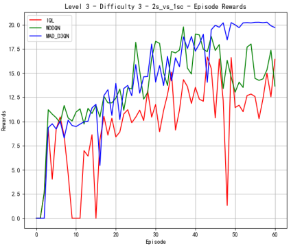
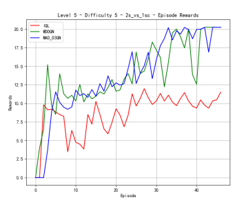
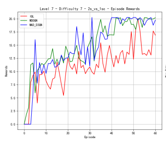
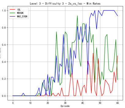
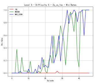
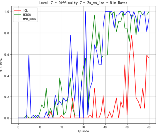
Figure 2. Comparison of reward and win_rate on map 2v_vs_1sc at different levels.

4.4. Results on map 3m

We also conduct the experiments on the map of 3m. As shown in Figure 3, our MAD-D3QN model quickly stabilizes rewards between 18.0 and 20 after approximately 15 episodes at the difficulty level of 3, while IQL struggles with rewards fluctuating around 10. This result shows the outstanding performance in multi agents reinforcement learning. Regarding the win rate metric, we obtain a peak value of nearly 1.0 after 20 epochs. The win rate of MADDQN fluctuates between 0.3 and 0.5, and IQL remains below 0.2. At difficulty level 5, our model consistently achieves rewards in the 17.5 to 20 range after 30 episodes, outperforming MADDQN, which stabilizes between 15 and 17.5. IQL continues to underperform, with rewards mostly fluctuating around 10. Regarding the win rates, our model reaches a near-perfect 1.0 win rate by episode 25 and maintains this high level, while MADDQN fluctuates between 0.4 and 0.7, and IQL nearly exceeds 0.2. For the most challenging case in Figure 3(c), we still outperform all the counterparts. Our rewards can quickly increase to 17.5 within 30 epochs, highlighting the robustness of proposed MAD-D3QN in handling complex scenarios. Compared to the MADDQN that achieves a reward around 15 but exhibits significant variability, our MAD-D3QN shows more stable reward stabilizing between 17.5 and 20. IQL remains consistently low with a reward generally below 10. Moreover, we achieve and sustain a win rate near 1.0 by episode 30, while MADDQN struggles with fluctuations between 0.3 and 0.6, and IQL rarely surpasses 0.2. All the results show the effectiveness of the proposed MAD-D3QN on map 3m.

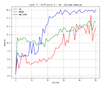
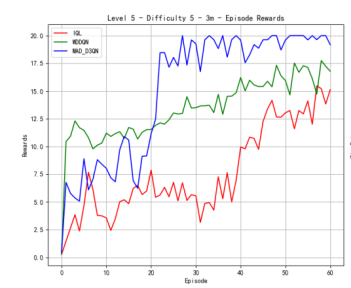
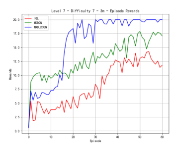
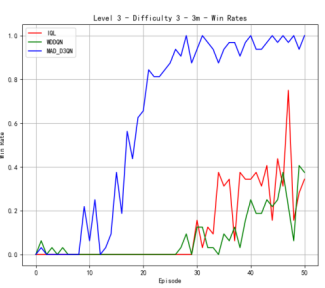
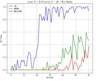
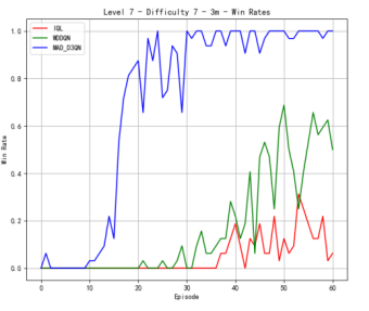
Figure 3. Comparison of reward and win_rate on map 3m at different levels.

4.5. Results on map 8m

Figure 4 shows our quantitative comparison with the state-of-the-art methods on more complex 8m. At difficulty level 3, the reward of MAD-D3QN rapidly increases to 20 during 30 epochs, while MADDQN shows a competitive reward stabilizing between 15 and 17.5. Our MAD-D3QN surpass the IQL more than 15 in the best reward. Similar gain trend can be observed in the win rates. At difficulty level 5, rewards of our model keep stable between 17.5 and 20 after 30 episodes, while MADDQN stabilizes slightly lower experiences notable fluctuations with a limited reward around 15. The win rates show that out model achieves better performance by episode 30, maintaining a win rate close to 1.0. In the last stage, facing the highest difficulty, our model displays its superiority successfully, where rewards quickly rise and stabilize between 17.5 and 20 by episode 35. For MADDQN, its rewards can reach 20 but have difficulty maintaining the value, while IQL only exceeds rewards of 12.5 to 15. Also, the win rates show the dominance of our model, as it reaches near 1.0 by episode 30, whereas MADDQN fluctuates more widely between 0.7 and 0.9, and IQL remains mostly flat around 0.4. Across different maps, we can achieve a consistent performance gain, demonstrating the effectiveness and robustness of our proposed MAD-D3QN.

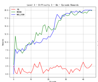
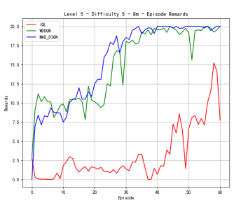
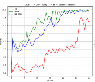
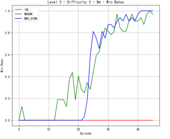
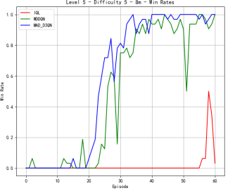
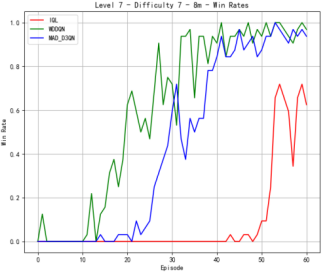
Figure 4. Comparison of reward and win_rate on map 8m at different levels.

4.6. Quantitative Comparison with SOTA methods

We finally report the best reward and win rate of our method on different maps in Table 1. For a fair comparison with previous methods, we fix the training step with a value of 25000 at the most challenging difficulty level 7. We obtain 100% win rate on map 2_vs_1c and map 3m, which outperforms the MADDQN by 15.7% and 31.3%, respectively. When the scene changes to more complex map 8m, our win rate is lower than MADDQN within the same training steps. We suppose the possible reasons may come from our dual attention mechanism, where training such complex network cost more computational overhead. However, our reward values consistently outperform on different maps, indicating the effectiveness of our collaborative strategy, which encourages different agents to consider the actual situation of other agents while maximizing their own performance, thereby maximizing the overall quality of network environment interaction. All the above results indicate the effectiveness of our method.

Table 1. Rewards and win_rates at fixed 250000 time steps

5. Conclusion

This paper proposes a MAD-D3QN model for better decision-making in Multi-Agent reinforcement learning. The model enables accurate Q-value calculation, with multi-layer attention mechanisms that can dynamically change state value and action advantage weights suitable in complicated multi-agent environments to construct a dynamic D3QN. Furthermore, it effectively learns from trajectories with higher rewards based on TD error, thereby focusing more on better-quality trajectories during training. Our model effectively mitigates the overestimation bias and discerns the intrinsic value of a state independently of the selected action, making more informed and effective decision-making processes. We evaluated it in multiple settings across different StarCraft II maps with various numbers of agents and difficulty levels. The experiment results demonstrate that the model can improve policy flexibility and efficiency while also achieving stronger adaptation ability in complex adversarial environments.

References

[1]. Mnih, V., Kavukcuoglu, K., Silver, D., Rusu, A. A., Veness, J., Bellemare, M. G., Graves, A., Riedmiller, M., Fidjeland, A. K., Ostrovski, G., Petersen, S., Beattie, C., Sadik, A., Antonoglou, I., King, H., Kumaran, D., Wierstra, D., Legg, S., & Hassabis, D. (2015). Human-level control through deep reinforcement learning. Nature, 518(7540), 529-533.
[2]. Hafiz, A. M., & Bhat, G. M. (2020). Deep Q-Network based multi-agent reinforcement learning withbinary action agents. arXiv preprint arXiv:2008.04109.
[3]. Rashid, T., Samvelyan, M., de Witt, C. S., Farquhar, G., Foerster, J., & Whiteson, S. (2018). QMIX: Monotonic value function factorisation for deep multi-agent reinforcement learning. Proceedings of the 35th International Conference on Machine Learning, PMLR, 80, 4292-4301.
[4]. Sunehag, P., Lever, G., Gruslys, A., Czarnecki, W. M., Zambaldi, V., Jaderberg, M., ... & Blundell, C. (2018). Value-decomposition networks for cooperative multi-agent learning. arXiv preprint arXiv:1706.05296.
[5]. He, Y., Mu, C., & Sun, Y. (2023). Enhancing Intersection Signal Control: Distributional Double Dueling Deep Q-learning Network with Priority Experience Replay and NoisyNet Approach. 2023 19th International Conference on Mobility, Sensing and Networking (MSN), Mobility, Sensing and Networking (MSN), 2023 19th International Conference on, MSN, 794–799. https://doi-org.ez.xjtlu.edu.cn/10.1109/MSN60784.2023.00116
[6]. Zhang, K., Yang, Z., & Başar, T. (2019). Multi-Agent Reinforcement Learning: A Selective Overview of Theories and Algorithms.
[7]. Lou, Z., Wang, Y., Shan, S., Zhang, K., & Wei, H. (2024). Balanced prioritized experience replay in off-policy reinforcement learning. Neural Computing and Applications, 36(25), 15721–15737. https://doi-org.ez.xjtlu.edu.cn/10.1007/s00521-024-09913-6
[8]. Rashid, T., Samvelyan, M., de Witt, C. S., Farquhar, G., Foerster, J., & Whiteson, S. (2020). Monotonic Value Function Factorisation for Deep Multi-Agent Reinforcement Learning.
[9]. Kallinteris, A., Orfanoudakis, S., & Chalkiadakis, G. (2024). A comprehensive analysis of agent factorization and learning algorithms in multiagent systems. Autonomous Agents & Multi-Agent Systems, 38(2), 1-48.
[10]. Foerster, J., Farquhar, G., Afouras, T., Nardelli, N., & Whiteson, S. (2018). Counterfactual multi-agent policy gradients. Proceedings of the AAAI Conference on Artificial Intelligence, 32(1).
[11]. Yu, W., Wang, R., & Hu, X. (2023). Learning Attentional Communication with a Common Network for Multiagent Reinforcement Learning. Computational Intelligence & Neuroscience, 1–12. https://doi-org.ez.xjtlu.edu.cn/10.1155/2023/5814420
Cite this article
Jiang,J. (2024). Adaptive Multi-layer Attention Double Dueling Deep Q-Network for Muti-agent Reinforcement Learning. Applied and Computational Engineering,103,211-219.
Data availability
The datasets used and/or analyzed during the current study will be available from the authors upon reasonable request.
Disclaimer/Publisher's Note
The statements, opinions and data contained in all publications are solely those of the individual author(s) and contributor(s) and not of EWA Publishing and/or the editor(s). EWA Publishing and/or the editor(s) disclaim responsibility for any injury to people or property resulting from any ideas, methods, instructions or products referred to in the content.
About volume
Volume title: Proceedings of the 2nd International Conference on Machine Learning and Automation
© 2024 by the author(s). Licensee EWA Publishing, Oxford, UK. This article is an open access article distributed under the terms and
conditions of the Creative Commons Attribution (CC BY) license. Authors who
publish this series agree to the following terms:
1. Authors retain copyright and grant the series right of first publication with the work simultaneously licensed under a Creative Commons
Attribution License that allows others to share the work with an acknowledgment of the work's authorship and initial publication in this
series.
2. Authors are able to enter into separate, additional contractual arrangements for the non-exclusive distribution of the series's published
version of the work (e.g., post it to an institutional repository or publish it in a book), with an acknowledgment of its initial
publication in this series.
3. Authors are permitted and encouraged to post their work online (e.g., in institutional repositories or on their website) prior to and
during the submission process, as it can lead to productive exchanges, as well as earlier and greater citation of published work (See
Open access policy for details).