1. Introduction

Nowadays, in the competitive used car market, accurately predicting vehicle prices is not just for convenience—it is necessary for consumers, dealers, and online marketplaces. In car price predicting, many models were developed, increasing the accuracy of the prediction. Among these models, Multi-linear regression works best[1]. Multi-linear regression model will be the main model to discuss in car price predicting in the future. Therefore, studying and understanding linear regression model in car price predicting is essential. This essay uses machine learning techniques to build a model which can accurately predict the used car price. Since Linear Regression is one of the fundamental models in predicting price[2], the paper will mainly discuss this model to predict the prices of used cars based on a comprehensive dataset which is available on Kaggle.com[3]. The dataset, which includes various attributes like make, odometer, and condition, provides a good platform for building an accurate model to predict the used car price.

The primary goal of this essay is to develop and analyze linear regression model that not only forecasts used car prices with a high degree of accuracy but also provides possible improvements of the model. This study focuses on showing the practical applications of machine learning techniques in real-world scenarios, which will highlight both their strengths and limitations. Through this exploration, the essay will contribute to the broader discourse on the integration of data science and machine learning in automotive industry. In addition, with the development of machine learning, many encoding strategies, like one-hot, labeling, are developed, but all of the strategies have disadvantages. Thus, this essay also want to find or develop a relative better encoding strategy to increase the prediction accuracy.

2. Methodology

2.1. Data preprocessing

This study uses a comprehensive dataset from Kaggle.com, with name “Used Car Dataset”. This dataset comprises a huge amount of entries representing individual cars. Each entry in the dataset includes several features which is relevant to the car’s market value, such as, Year (Entry Year), Model (Model of Vehicle), Condition (Condition of Vehicle), and Cylinder (Number of Cylinders). Because of the diverse of features, the dataset can provide a strong foundation for predicting vehicle prices through machine learning techniques. The preparation of the dataset involves several critical steps to ensure the data is suitable for modeling.

2.1.1. Feature selection

Certain columns in the dataset, such as ‘id’, ‘url’, ‘VIN’, ‘image_url’, and ‘description’, will not provide valuable information for prediction. Thus, these columns were removed.

2.1.2. Filtering outliers in price and year

The paper used a specific criterion for filtering out price outliers by keeping vehicle prices within the range from $1,000 to $100,000. Additionally, prices are scaled down by 1000, simplifying the model’s numerical computations and increasing the interpretability.

A filter were implemented on year to include only vehicles from 2000 to the newest to focus on recent transactions.

2.1.3. Handling missing and ambiguous values

To preserve the potential distribution, the missing values are removed. Entries with value of ‘other’ in all fields are also removed since “other” provides unclear information.

2.1.4. Convert categorical date to numerical data

This paper used two strategies for converting, one is label-encoding[4], and another is mixed strategy.

For mixed strategy, for ordinal data, where categories have a natural order, such as ‘condition’ (from ‘salvage’ to ‘new’), this paper will apply manual mapping. This involves assigning each category a unique integer based on its relative ranking. For nominal categorical variables, such as ‘color’, this paper uses one-hot encoding. This method transforms each category into a new binary column, ensuring that the model treats each category distinctly without imposing any ordinal relationship[5].

2.2. Model development and evaluation

The development of the linear regression model followed a traditional approach to ensure the accuracy and reliability. To construct and evaluated the models, the first step is model training; then the next step is to evaluate it.

(1).Model Training:

The encoded datasets were split into training (80%) and testing (20%) sets using a consistent random seed(0). Linear regression models were then trained on the encoded datasets.

(2).Model Evaluation:

The models were evaluated by the Mean Squared Error (MSE) and R-squared values.

Table 1: Performance Matrix of Linear Regression.

(3).Interpretation and Analysis

The results indicate the mixed encoding strategy is superior effectiveness over the label encoding. By treating nominal and ordinal data distinctly—preserving the categorical nature through one-hot encoding for nominal and label encoding for ordinal—this strategy enhances predictive accuracy and model interpretability. From Table 1, the R-squared value of 0.70 for mixed strategy indicates that about 70% of the variability in the actual prices can be explained, which is generally considered as a strong effect size[6], a “good” value, higher than 0.63. Thus, the mixed strategy will be focused in the following part.

In Figure1, the blue dots represent actual prices of vehicles, while the points on the red dashed line indicate perfect predictions where the predicted prices perfectly match the actual prices. The closer the blue dots are to the red line, the more accurate the model’s predictions. According to this figure, a dense cluster of points along the red line suggests that for a majority of the data, the model's predictions are close to the actual prices, indicating a good overall fit. However, at the higher price level, the linear regression model has underestimating problems. In Figure2, the blue dots represent actual prices of the vehicles, and the red dots represent predicted prices by the linear regression model. These dots show the distribution of the actual price and predicted price. This figure also indicates that at lower price level, the fitting is pretty good, and the model has underestimating problem at higher price level. The occurrence of negative predicted prices, as observed in Figure1 and Figure2, highlights critical limitations. Since negative prices are not feasible in the real life, this points the potential areas for model refinement. Adjustments may include transforming the target variable to better accommodate the non-linear distribution or applying more robust regression techniques that constrain predictions to non-negative values.

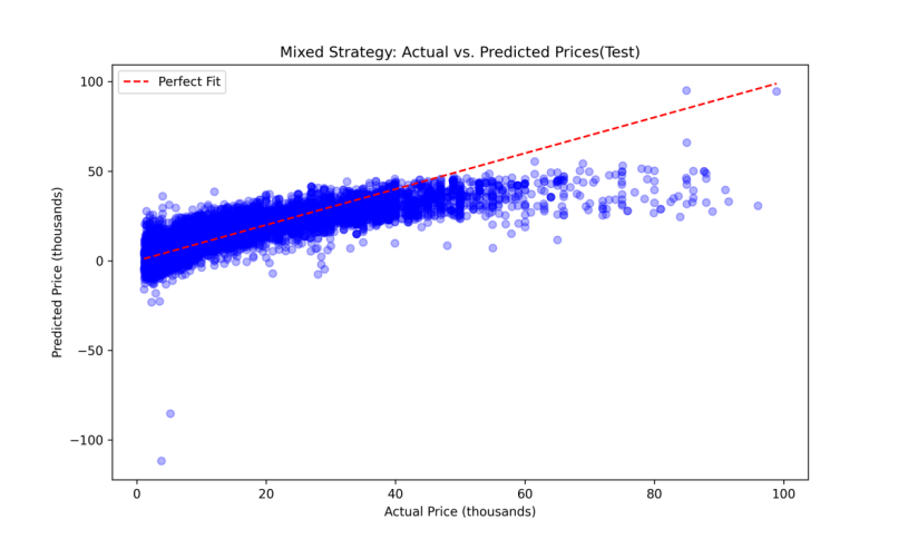
Figure 1: Mixed Strategy: Actual vs. Predicted Prices(Test)(LR).

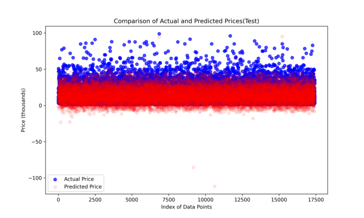
Figure 2: Comparison of Actual and Predicted Prices(Test)(LR).

As Table 1 shows, an MSE of 44.02 for mixed strategy indicates the average squared difference between the actual and predicted prices. From both Figure1 and Figure2, the fit is pretty good for lower price. However, at higher price levels, the plots show that the fit is not perfect, which means the model tends to under-predict prices. This deviation suggests that the model may not fully capture the factors that drive higher vehicle values, or at higher price levels, the relationship between features and price is not linear.

3. Analysis

3.1. Decision tree performance

To assess the robustness and adaptability of the model, the performance of decision tree model will be compared to the Linear Regression model using the same dataset and feature encoding strategies, in addition same random seed.

Model Evaluation:

The models were evaluated using the Mean Squared Error (MSE) and R-squared values.

Table 2: Performance Matrix of Decision Tree.

3.2. Analysis and comparison

Based on Table2, the mixed strategy will be focused. From Table2, Decision Tree model's training R-squared value of 1.00 and MSE of 0.02 suggest that the model perfectly fits the training data. The model demonstrated notably higher predictive accuracy and data fit compared to the previously analyzed Linear Regression model. In testing, by using mixed encoding strategy, the Decision Tree model could achieve an R-squared value of 0.84, signifying that it could explain approximately 84% of the variability in vehicle prices. This is a marked improvement over linear regression model.

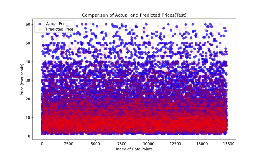
Figure 3: Comparison of Actual and Predicted Prices(Test)(DT).

Moreover, as Table 2 showed, the MSE of 23.65 for the Decision Tree model in testing represents a substantial decrease from the linear model’s MSE, highlighting a more precise prediction. This lower MSE underscores the model’s effectiveness in minimizing the error magnitude between the predicted and actual prices.

Figure3 contains similar information as Figure2 provided, but now the predicted prices are from decision tree model. Figure3 shows a almost perfect fit.

Figure4 contains similar information as Figure1 provided, but now the predicted prices are from decision tree model. Figure4 shows a almost perfect fit.

The Figure3 shows a tighter clustering of predictions around the actual prices, indicating that the Decision Tree model may be more effective in accurately predicting price. This trend is evident in the Figure4, which shows a closer alignment along the perfect fit line, especially in the lower to mid-price range.

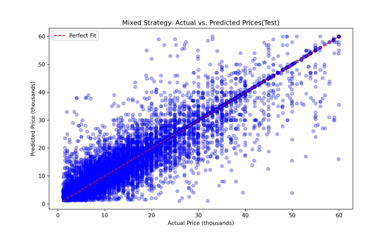
Figure 4: Mixed Strategy: Actual vs. Predicted Prices(Test)(DT).

However, the perfect fitting is not always a good news. Such a high R-squared value may imply overfitting. Overfitting leads to less robust models that perform well on training data but poorly on new, unseen data i.e. large gap between training and test error[7]. This can be problematic in real-world applications where flexibility and adaptability to new data are crucial. The analysis of the Decision Tree model indicates a potential issue of overfitting, which is suggested by the stark difference between the training and testing performance metrics. From Table 2, the Decision Tree model's training R-squared value of 1.00 and MSE of nearly 0.02 suggest that the model perfectly fits the training data. While at first glance this might appear ideal, it actually raises concerns about the model's generalization ability. A perfect fit to the training data often implies that the model has not only learned the underlying patterns but also the noise specific to the training set. While the testing R-squared of 0.83 and MSE of 24.13 still indicate strong performance, the discrepancy between the training and testing results is a hallmark of overfitting. The model's performance on unseen data is notably worse compared to the training set. This degradation suggests that the model may be too complex, capturing intricate details that do not generalize to new data.

Unlike the Decision Tree, Linear Regression model shows less discrepancy between its training and testing performance, indicating a more stable and consistent model that might be less prone to overfitting. Thus, the Linear Regression model shows a better generalizability in predicting car price.

In conclusion, at lower price level, the Linear Regression model will be the best choice since from the plot the model performs very well at lower price level. At higher price level, the Decision Tree model will be better if the overfitting problems can be disproved since the Linear Regression model has under-predict issues.

4. Discussion

4.1. Implications in the context of vehicle pricing

The performance of both the Decision Tree and Linear Regression models has significant implications for vehicle pricing strategies in a real-world setting. For the Decision Tree model, the model has a very high accuracy and an excellent fit of the data. This suggests that the Decision Tree model can be highly effective for predicting vehicle prices based on their attributes. However, one must be careful when using this model as it may have overfitting problems. In the realm of vehicle pricing prediction, overfitting can have significant practical implications. Decision Tree models that overfit the training data might appear to offer high precision during the development phase but could ultimately lead to unreliable price estimations when applied in real-world scenarios.

Thus for Linear Regression model, with great generalizability and excellent performance at lower price level, one could use this model very confidently. However, at higher price level, especially above $60,000, this model performs much worse than the Decision Tree model, thus, leading to unreliable price frequently. In addition, the Linear Regression model may give some negative prediction values when it makes predictions at the super low price level. If a predictive model is used by a dealership or an online pricing tool overestimating or underestimating vehicle prices due to overfitting or under-predicting, it will lead to discrepancies between predicted prices and market realities. This disparity can erode consumer trust and satisfaction, since customers may miss out on fair deals. Dealers will also rely on accurate price predictions for inventory purchasing and pricing strategies. Unreliable pricing can lead to forecasting errors, which may result in dealers purchasing inventory that does not match market demand or pricing vehicles in a way that drives away potential buyers, which may cause unnecessary losses.

Thus, for cars that generally have a price lower than $60,000, using Linear Regression model would be a better choice. For cars that generally have price higher than $60,000, people may use Decision Tree model with care.

4.2. Limitation and improvements of linear regression model

Linear regression assumes a linear relationship between independent and dependent variables. This assumption often doesn’t hold in complex scenarios like vehicle pricing where the relationships might be non-linear due to factors such as brand value, unexpected market trends, or unique vehicle features. In this case, utilizing polynomial regression or transforming variables can help capture non-linear relationships. More complex models like Random Forest or Neural Networks might also be appropriate, but one needs to be careful with overfitting problems. In addition, linear regression models are sensitive to outliers. Outliers can have a disproportionately large effect on the fit of the model, leading to skewed results which might not truly represent the general trend of the data. For this, Robust Regression can be used to reduce the effect of outliers because this model uses a method called iteratively re-weighted least squares to assign a weight to each data point[8]. Linear regression can predict negative values, which are not feasible in contexts like vehicle pricing. To prevent non-sensical negative predictions, models could be constrained to non-negative outputs. Implementing transformations such as logarithmic transformation of the target variable can also be an effective solution.

5. Conclusion

This section focuses on the key findings on linear regression model. The application of linear regression to predict vehicle prices has yielded several critical insights, which indicate a substantial fit of the model for practical applications. The model’s predictive accuracy in terms of MSE represents the average squared difference between the actual prices and the predicted prices, providing a quantitative measure of the model’s performance. When people use linear regression model to predict, the strategy of encoding the categorical data to numerical data is essential. This essay showed mixed strategy will be a good choice. Since one-hot encoding will not preserve the ordinal properties of categorical data, like the ‘condition’, if people only use this strategy, some information which could increase the accuracy of our prediction may be lost. On the other hand, if people only use label encoding, some incorrect information may be introduced, like for nominal data, using label encoding will automatically introduce ordinal relationship, which will cause bias. Thus, in most cases, mixed strategy will always be a good option for pursuing the accuracy.

The exploration and findings from the linear regression model in this essay contains some drawbacks. The dataset used by this essay contains lots of missing values, so simply dropping the columns with missing values may cause the lost of useful information. Future work may include finding an algorithm to assign values to the missing value. Also, this essay did not explore the relationship between car price and every other feature of the vehicle, like relationship between price and mileage. Additionally, because of mixed encoding strategy, the dimensionality is large. Future studies could explore non-linear transformations of the input features or the target variable (e.g., logarithmic or square root transformations) to better capture the complex relationships within the data and address issues like negative price predictions. Since the model used by essay has not been used by consumers and dealers, to validate the model’s practical utility, further testing in real-world scenarios or deployment in a live environment could be conducted.

References

[1]. R. Swarnkar, R. Sawant, H. R and S. P. (2023) Multiple Linear Regression Algorithm-based Car Price Prediction, 2023 Third International Conference on Artificial Intelligence and Smart Energy (ICAIS), Coimbatore, India, pp. 675-681
[2]. Kumar, S., & Sinha, A. (2024). Predicting Used Car Prices with Regression Techniques. International Journal of Computer Trends and Technology, 72(6), 132–141.
[3]. AUSTIN REESE. (2021). Used Cars Dataset. https://www.kaggle.com/datasets/austinreese/craigslist-carstrucks-data/data
[4]. VITALII MOKIN. (2019). Used Cars Price Prediction by 15 models. https://www.kaggle.com/code/vbmokin/used-cars-price-prediction-by-15-models#6.-Models-comparison-.
[5]. Vasques, X. (2024). Machine learning theory and applications: hands-on use cases with Python on classical and quantum machines.
[6]. Moore, D. S., Notz, W. I, & Flinger, M. A. (2013). The basic practice of statistics (6th ed.). W. H. Freeman and Company, New York. pp.138.
[7]. Syam, Niladri, Rajeeve Kaul. (2021). Overfitting and Regularization in Machine Learning Models. Machine Learning and Artificial Intelligence in Marketing and Sales: Essential Reference for Practitioners and Data Scientists. 1st ed. Emerald Publishing Limited. Bingley. pp.14.
[8]. Robert Andersen. (2008) Robust Regression for the Linear Model. Modern Methods for Robust Regression. SAGE Publications, Inc. pp.48-70.
Cite this article
He,J. (2024). Predicting Vehicle Prices Using Machine Learning: A Case Study with Linear Regression. Applied and Computational Engineering,99,35-42.
Data availability
The datasets used and/or analyzed during the current study will be available from the authors upon reasonable request.
Disclaimer/Publisher's Note
The statements, opinions and data contained in all publications are solely those of the individual author(s) and contributor(s) and not of EWA Publishing and/or the editor(s). EWA Publishing and/or the editor(s) disclaim responsibility for any injury to people or property resulting from any ideas, methods, instructions or products referred to in the content.
About volume
Volume title: Proceedings of the 5th International Conference on Signal Processing and Machine Learning
© 2024 by the author(s). Licensee EWA Publishing, Oxford, UK. This article is an open access article distributed under the terms and
conditions of the Creative Commons Attribution (CC BY) license. Authors who
publish this series agree to the following terms:
1. Authors retain copyright and grant the series right of first publication with the work simultaneously licensed under a Creative Commons
Attribution License that allows others to share the work with an acknowledgment of the work's authorship and initial publication in this
series.
2. Authors are able to enter into separate, additional contractual arrangements for the non-exclusive distribution of the series's published
version of the work (e.g., post it to an institutional repository or publish it in a book), with an acknowledgment of its initial
publication in this series.
3. Authors are permitted and encouraged to post their work online (e.g., in institutional repositories or on their website) prior to and
during the submission process, as it can lead to productive exchanges, as well as earlier and greater citation of published work (See
Open access policy for details).