1. Introduction

In recent times, global stock markets have experienced notable declines. Of particular note is the fact that the Nikkei 225 experienced its most significant single-day decline in decades, with a drop exceeding 12%. This market turbulence serves to illustrate the vulnerability of global financial systems to abrupt policy changes and economic uncertainty [1]. In response to this turbulence, investors have exhibited a range of reactions, with many displaying heightened anxiety. In the context of the prevailing economic conditions, an increasing number of individuals are employing stock prediction models with the objective of mitigating the risk and failure rate of stock investments. These models integrate advanced machine learning techniques like neural networks and random forests with statistical methods like ARIMA and Generalized Autoregressive Conditional Heteroskedasticity (GARCH). These techniques analyze historical data, market trends, and other variables in order to predict potential price movements. It should be noted, however, that the stock forecasting model is not infallible and may be subject to certain limitations. These include the potential for market unpredictability, data quality issues, and overfitting, which could result in inaccurate forecasts and financial losses in highly volatile or unprecedented market conditions. In order to minimize losses and to the greatest extent possible, align the interests of shareholders with those of the organization, this essay will first introduce the stock forecasting models proposed by predecessors and provide an analysis of their shortcomings. It will then proceed to provide a comprehensive explanation of the ARIMA model, demonstrating its practical applicability through the use of an illustration.

2. The Review of Stock Forecasting Models

2.1. The Long Short-Term Memory (LSTM) network

Firstly, a substantial body of research has been conducted on stock forecasting models by predecessors, with a number of notable studies emerging from this work. One particularly notable example is the Long Short-Term Memory (LSTM) network, which was first introduced by Hochreiter and Schmidhuber [2]. It addresses the limitations of traditional recurrent neural networks (RNNs), particularly their difficulty in processing long-term dependencies due to the vanishing gradient problem. LSTMs incorporate gating mechanisms, comprising input, forget, and output gates, which regulate information flow. This makes them highly effective for tasks involving sequential data, such as natural language processing (NLP), speech recognition, and time series forecasting. These models have become a fundamental component in NLP applications, including machine translation and text generation [3]. They have also demonstrated superior performance compared to traditional models in speech recognition [4]. Subsequently, several variations of the LSTM have been proposed, including the Gated Recurrent Unit (GRU), which simplifies the model by merging the forget and input gates into a single update gate [5]. In the field of stock market forecasting, LSTMs have demonstrated potential due to their capacity to capture the temporal dependencies and non-linear patterns inherent to financial time series. However, their computational complexity, particularly when training on large datasets or deploying in real-time systems, represents a notable limitation. Furthermore, LSTMs are prone to difficulties when processing extremely lengthy sequences.

2.2. The Transformer Network

Transformers, as proposed by Vaswani et al. [6] represent a significant advancement in the processing of sequential data. They offer a solution to the inherent limitations of existing models, such as RNNs and LSTMs, which process input data sequentially and are susceptible to vanishing gradient issues. Transformers eschew reliance on sequential processing, instead leveraging a self-attention mechanism that allows the model to focus on different parts of the input sequence simultaneously. This parallelisation capability enables transformers to capture long-range dependencies in the data with greater efficiency, rendering them particularly powerful for tasks involving complex sequences. The self-attention mechanism has been demonstrated to constitute a significant advancement, resulting in the development of highly successful models such as BERT (Bidirectional Encoder Representations from Transformers) and GPT (Generative Pretrained Transformer). These have become foundational in the field of natural language processing (NLP) [7]. Nevertheless, the computational demands of transformers are considerable, as the self-attention mechanism scales quadratically with input length. Additionally, transformers necessitate a considerable quantity of data for optimal functionality, which poses difficulties in domains with limited data availability [8].

2.3. The AutoRegressive Integrated Moving Average (ARIMA)model

The ARIMA (AutoRegressive Integrated Moving Average) model is a widely used statistical method for time series forecasting. It offers a traditional linear approach that contrasts with more complex deep learning models, such as LSTMs and transformers. One of the key advantages of ARIMA is its interpretability and lower computational requirements, which render it particularly effective in scenarios where data is limited or more complex models may be unnecessary. Therefore, the model is particularly well-suited to applications that require a clear insight into the relationships within the data [9]. The three principal components of ARIMA are autoregression (AR), differencing (I), and moving average (MA). The autoregressive (AR) component is used to model the relationship between an observation and its preceding values, thereby capturing the influence of past values on the current one. The integrated component, or differencing, addresses the issue of non-stationarity by transforming the series into a stationary one, which is a crucial step in the effective modeling process. In contrast, the moving average (MA) component models the relationship between an observation and the residual errors from a moving average model, allowing ARIMA to account for short-term fluctuations in the data. The flexible structure of ARIMA allows it to model a wide variety of time series, making it particularly useful for short-term forecasting. For instance, financial markets can use ARIMA to identify patterns in stock prices or interest rates. Observable time dependencies in these areas often display predictable patterns. ARIMA's ability to model such dependencies with a relatively simple framework provides an effective solution in cases where more advanced machine learning models may be too resource-intensive or infeasible. Therefore, ARIMA continues to be a valuable and practical tool in numerous forecasting applications, particularly in situations where computational resources or large datasets are scarce.

3. Predicting the rise and fall of stocksusing ARIMA model

3.1. Load data

First, get the trading data of the CSI 300 index from 2012 to 2022 from the Kaggle website. The CSI 300 represents a significant indicator of the Chinese financial market, comprising the 300 largest stocks in China by market capitalisation. This dataset collates trading data for these 300 stocks over the course of the 2022 financial year. Subsequently, the Python code, which is structured to facilitate the analysis of stock market data, specifically from a dataset named `data.csv`, is utilised. This code performs several key tasks, including importing necessary libraries, configuring visualisation settings, and loading the dataset for further analysis.

3.1.1. Library Imports

The code commences with the importation of a number of fundamental Python libraries. The `pandas` library (imported as `pd`), in particular, is employed for the manipulation and analysis of tabular data. The data visualisation tools `seaborn` and `matplotlib. pyplot` (imported as `sns` and `plt`, respectively) are employed for the creation of detailed and informative plots. The `statsmodels. api` module (imported as `sm`) is included for the purpose of statistical modeling, which is likely to be employed in subsequent stages of the analysis. To avoid non-critical warning messages cluttering the output during execution, the command `warnings.filterwarnings('ignore')` is used.

3.1.2. Visualization Settings

The code configures seaborn and matplotlib to utilise the "SimHei" font, thereby ensuring the accurate rendering of Chinese characters within the plots. By correctly displaying negative signs in plots, the configuration plt.rcParams ['axes. unicode_minus'] = False ensures the accurate representation of data.

3.1.3. Data loading

The variable `stock_file` is used to store the file path to the stock data, in this case, `data.csv`. Subsequently, the data is loaded into a Pandas DataFrame (df) using pd.read_csv(). The trade_date column is designated as the index and is parsed as datetime objects, which is essential for time series analysis. Treating the data as a time-indexed series facilitates operations like trend analysis, forecasting, and other temporal analyses.

3.1.4. Output

Ultimately, the code outputs the contents of the DataFrame, `df`, thereby enabling the user to examine the loaded data and confirm that it has been correctly processed and indexed.

3.2. Data preprocessing

In order to forecast the closing price, the closing price data is resampled and averaged on a weekly basis, with the specified Monday included. The data from January 2013 to December 2022 is then designated as the training data, which is subsequently displayed visually.

The objective of this Python code is to analyse and forecast stock closing prices using resampling and visualisation techniques. The stock price data is resampled with a focus on the `close` column, with weekly averages calculated (`stock_week = df['close'].resample('W-MON').mean( )`). This process simplifies the data, allowing for the identification of trends over time. This resampled data is filtered to include only the period from January 2013 to December 2022 (`stock_train = stock_week['2013-1':’2022-12']`), thereby creating a focused dataset for training and analysis. At last, a line plot, which is figure 1, is generated to illustrate the weekly trends (`stock_train.plot(figsize=(15,6))`), with the plot's appearance refined using the `sns.despine()` function.

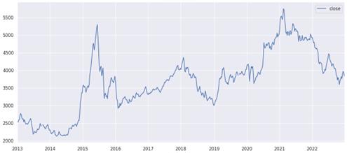
Figure 1. Average Weekly Closing Price Graph 2013-2022.

3.3. Difference and determine the parameter: d

The purpose of data splitting is to ensure the data set's stationarity, as evidenced by the substantial fluctuations observed in the original data set that necessitate the implementation of a splitting operation. After two rounds of splitting, the data are presented for visual inspection.

The Python code presented here performs differencing on a time series with the objective of stabilising its mean by removing trends. This is a crucial step in preparing the data for time series forecasting models such as ARIMA. The code specifically addresses the process of determining the differencing parameter, represented by the letter 'd', which indicates the number of times the data must be differenced in order to achieve stationarity.

3.3.1. First-Order Differencing

The initial line of code, `stock_diff_1 = stock_train.diff()`, performs the calculation of the first-order differences of the `stock_train` time series. This is achieved by subtracting each observation from the previous one, thereby removing linear trends. The subsequent line of code, `stock_diff_1.dropna(inplace=True)`, removes any `NaN` values generated due to differencing at the outset of the series. The following section presents the results of the first-order differencing process.

3.3.2. Second-Order Differencing

Subsequently, the code performs second-order differencing with `stock_diff_2 = stock_diff_1.diff( )`, which involves differencing the already differenced data (`stock_diff_1`). This step serves to further stabilise the series in the event that the first-order differencing was insufficient. Once more, the code removes any NaN values generated by this additional differencing with the command `stock_diff_2.dropna(inplace=True)`.

3.3.3. Visualisation

To visualize the effects of differencing, the code generates a figure consisting of two subplots. The initial subplot, designated as `plt.subplot(2,1,1)`, depicts the first-order differenced series (`stock_diff_1`) and is labeled "First-Order Differencing." The second subplot (`plt.subplot(2,1,2)`), which is labelled "Second-Order Differencing," plots the second-order differenced series (`stock_diff_2`). Subsequently, the `plt.show()` command displays the plots, allowing for a visual inspection of the differenced series to determine whether it has been adequately transformed to achieve stationarity.

The following two figures are the resulting figures 2 and 3

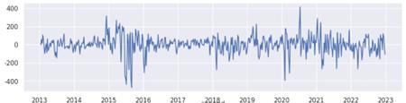
Figure 2. First order difference diagram.

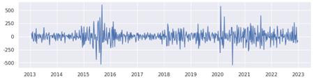
Figure 3. Second order difference diagram.

This process is pivotal in time series analysis, as it facilitates the identification of the requisite differencing order, denoted by the variable d, which is necessary to prepare the data for modeling. This ensures that the series meets the assumptions required for accurate forecasting. The figure above illustrates that the first-order difference has undergone a shift from a stable trend, and the amplitude of the second-order fluctuation is even more pronounced. Consequently, we can ascertain with certainty that the parameter d is equal to 1. Subsequently, the parameters q and p are identified through the construction of ACF and PACF diagrams, respectively.

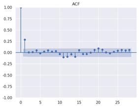
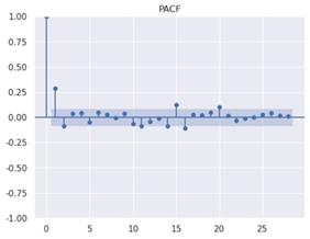
Figure 4. ACF diagram Figure 5. PACF diagram

The Python code generates and displays an autocorrelation function (ACF) plot for a first-order differenced time series, designated as "stock_diff_1." The ACF plot is generated using the `plot_acf` function from the `statsmodels` library, specifically from its `tsa` (time series analysis) module. This plot is of great importance for the visualisation of the correlation between the time series and its lagged values over a variety of time intervals. This enables the identification of significant patterns and the determination of the most appropriate lag parameters for models such as ARIMA. The plot is titled "ACF" for clarity, and the command `plt.show()` is used to render the plot, thus allowing for immediate visual inspection of the autocorrelations present in the data.

The figure shows that when the numerical anomaly of the ordinate corresponding to the point whose abscissa value is 1 is high, the optimum value of parameter q is 1. Similarly, the PACF diagram was constructed, and it was determined that the optimal parameter value of p is also 1.

3.4. Train the model and predict

Then, the ARIMA model is employed to forecast the time series and present the findings in a graphical format. The initial step is to construct an ARIMA model for the `stock_train` dataset, utilising the parameters `(1, 1, 1)` and a frequency setting of `'W-MON'`, which denotes weekly data commencing on Mondays. Subsequently, the model is fitted to the data set using the `fit()` method, resulting in a model object stored in the variable `result`. Subsequently, the code generates a forecast utilising the fitted model, with predictions commencing on 10 January 2022 and extending to 1 June 2023 (`forecast = result.predict(start='2022-12-10', end='2023-6-01')`). For purposes of visualisation, the code establishes a plot, which is figure 6, with a figure size of 12 by 6 inches. The xticks are rotated by 45 degrees to enhance the legibility of the date labels on the x-axis. The forecast series, representing the predicted values, is plotted alongside the original stock_train data, which represents the actual observed values. Each line is labelled with the appropriate designation ('Predicted value' for predicted values and 'True value' for actual values), and a legend is added to distinguish between them. Finally, plt.show() displays the plot, allowing for visual comparison between the forecasted and actual values over the specified period.

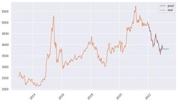
Figure 6. Time series prediction diagram of ARIMA model.

The model demonstrates a high degree of fit and is largely consistent with the original trend.

4. ARIMA model effect evaluation

The Python code creates diagnostic plots, figure 7, to assess the fit of an ARIMA model. The plot_diagnostics() method, when applied to the result object (which contains the fitted ARIMA model), produces a series of plots that assist in the evaluation of the model's underlying assumptions and performance. A residuals plot, a histogram or density plot of the residuals, a Q-Q plot to check if the residuals are normal, and an ACF plot to see if there is autocorrelation in the residuals are some of the diagnostics that are usually used.The argument `figsize=(16,12)` sets the dimensions of the figure, thereby ensuring that the diagnostic plots are of sufficient size for detailed examination. Finally, the command `plt.show()` is invoked to display these plots, thus enabling the analyst to visually inspect the model's diagnostics and determine whether the model is well-fitted or if any assumptions have been violated.

The provided image displays four diagnostic plots that were generated to evaluate the fit and assumptions of an ARIMA model applied to stock price data.

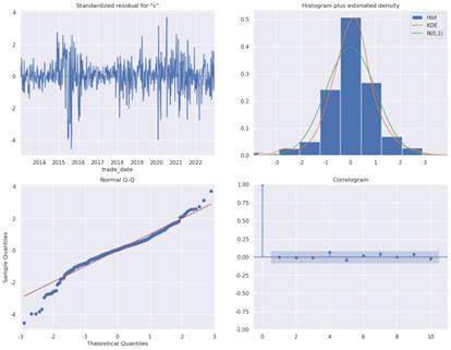
Figure 7. four diagnostic plots

The standardized residuals plot (top left) depicts the standardized residuals of the ARIMA model over time, with a mean of zero and a standard deviation of one. In an optimal scenario, the residuals would demonstrate random fluctuations around zero, lacking discernible patterns. This would indicate that the model has effectively captured the underlying data structure. The "Histogram plus Estimated Density" (top right) illustrates the distribution of the residuals, overlaid with a kernel density estimate (KDE) and a normal distribution curve (N(0,1)). This allows for the evaluation of whether the residuals are approximately normally distributed, which is a crucial assumption in ARIMA modeling. If the residuals exhibit a close adherence to the normal distribution (green curve), this indicates that the model is well-fitted. The "Normal Q-Q Plot" (bottom left) provides a graphical comparison of the residual quantiles with the expected quantiles of a standard normal distribution. If the residuals are normally distributed, the points will lie along the red line. Lastly, the correlogram (bottom right) illustrates the autocorrelation function (ACF) of the residuals. The blue bars represent correlations at varying lags, while the shaded region corresponds to the 95% confidence interval. If the residuals are white noise, the majority of autocorrelations will fall within this interval.

5. Conclusion

In conclusion, the ARIMA model represents a valuable analytical tool. LSTM models are good at detecting sequential dependencies and nonlinear patterns in stock data, and they work well for short-term forecasting. However, transformer networks, with their self-attention mechanism, can model long-range dependencies and complex interactions. They are particularly adept at handling large-scale financial data with complex temporal relationships. However, they are also subject to significant limitations. LSTM models may encounter difficulties when confronted with lengthy series and are computationally demanding, frequently resulting in the overfitting of financial data that is characterised by noise. Transformer networks are effective in capturing complex dependencies; however, they require substantial computational resources and large datasets, which may restrict their applicability in stock forecasting with limited data. In contrast, the ARIMA model is well suited to address these limitations and accurately predict stock price movements. The objective of the ARIMA model is to facilitate more informed purchasing and selling decisions, mitigate financial risk, and enhance returns. It is important to note, however, that all forecasts are based on the extrapolation of future trends and past periods. This implies that the future direction is not inherently predetermined. It is important to recognise that the ARIMA model has limitations when applied to non-linear models or long-term forecasting. In such cases, more sophisticated models may be required to achieve greater accuracy. Therefore, investors should adopt a rational and cautious approach, not relying too heavily on forecast results and remaining alert to actual developments. It should be noted that the financial markets are in a state of constant flux.

References

[1]. Martin, W., 2024. Here's Why Global Stock Markets Are on the Slide. Markets Insider. Available at: https://markets.businessinsider.com (Accessed: 15 August 2024).
[2]. Hochreiter, S. & Schmidhuber, J., 1997. Long short-term memory. Neural Computation, 9(8), pp. 1735-1780.
[3]. Sutskever, I., Vinyals, O. and Le, Q.V., 2014. Sequence to sequence learning with neural networks. In Advances in Neural Information Processing Systems (pp. 3104-3112).
[4]. Graves, A., Mohamed, A.-r. and Hinton, G., 2013. Speech recognition with deep recurrent neural networks. In 2013 IEEE International Conference on Acoustics, Speech and Signal Processing (pp. 6645-6649). IEEE.
[5]. Chung, J., Gulcehre, C., Cho, K. and Bengio, Y., 2014. Empirical evaluation of gated recurrent neural networks on sequence modeling. arXiv preprint arXiv:1412.3555.
[6]. Vaswani, A., et al., 2017. Attention is all you need. In Advances in Neural Information Processing Systems (pp. 5998-6008).
[7]. Tay, Y., Dehghani, M. and Bahri, D., 2020. Efficient transformers: A survey. arXiv preprint arXiv:2009.06732.
[8]. Box, G.E.P., Jenkins, G.M. and Reinsel, G.C., 2015. Time series analysis: forecasting and control. John Wiley and Sons.
Cite this article
Liu,X. (2024). Research on Auto Regressive Integrated Moving Average model in predicting the rise and fall of stocks. Applied and Computational Engineering,97,119-126.
Data availability
The datasets used and/or analyzed during the current study will be available from the authors upon reasonable request.
Disclaimer/Publisher's Note
The statements, opinions and data contained in all publications are solely those of the individual author(s) and contributor(s) and not of EWA Publishing and/or the editor(s). EWA Publishing and/or the editor(s) disclaim responsibility for any injury to people or property resulting from any ideas, methods, instructions or products referred to in the content.
About volume
Volume title: Proceedings of the 2nd International Conference on Machine Learning and Automation
© 2024 by the author(s). Licensee EWA Publishing, Oxford, UK. This article is an open access article distributed under the terms and
conditions of the Creative Commons Attribution (CC BY) license. Authors who
publish this series agree to the following terms:
1. Authors retain copyright and grant the series right of first publication with the work simultaneously licensed under a Creative Commons
Attribution License that allows others to share the work with an acknowledgment of the work's authorship and initial publication in this
series.
2. Authors are able to enter into separate, additional contractual arrangements for the non-exclusive distribution of the series's published
version of the work (e.g., post it to an institutional repository or publish it in a book), with an acknowledgment of its initial
publication in this series.
3. Authors are permitted and encouraged to post their work online (e.g., in institutional repositories or on their website) prior to and
during the submission process, as it can lead to productive exchanges, as well as earlier and greater citation of published work (See
Open access policy for details).