1. Introduction

Traffic flow forecasting is crucial for intelligent transportation systems (ITS), enabling effective traffic management, route optimization, and congestion reduction. The complex nature of traffic data, with its dynamic spatial-temporal dependencies and non-linear patterns, presents significant prediction challenges [1,2].

Conventional machine learning techniques, including time series and statistical models, often struggle to capture the non-linear and high-dimensional aspects of traffic data [2]. Recent advancements in deep learning have shown promise in addressing these issues [3]. While Convolutional Neural Networks (CNNs) and Recurrent Neural Networks (RNNs) have been applied to model spatial and temporal dependencies respectively [4,5], they may not adequately capture the intricate interplay between spatial and temporal dimensions in traffic data.

The use of Graph Neural Networks (GNNs) to model the relational structures in traffic networks represents a novel approach to representing road networks as graphs [6]. While GNN-based models like Diffusion Convolutional Recurrent Neural Networks (DCRNN) [5] and Graph WaveNet [7] have achieved notable success, they primarily focus on capturing spatial dependencies through graph convolutions and temporal dependencies through recurrent units or temporal convolutions separately.

In addition, attention mechanisms have been utilized in the context of traffic prediction with the goal of developing a dynamic model that accounts for dependencies. For instance, Spatial-Temporal Attention networks [8] and Graph Multi-Attention Networks (GMAN) [9] leverage attention to capture spatial-temporal correlations. Despite these advancements, existing models often handle spatial and temporal components in isolation or combine them in a sequential manner, which may limit their ability to fully exploit the multi-modal interactions present in traffic data. Specifically, the current studies highlight several limitations in recent traffic prediction models:

• Separate Modeling of Spatial and Temporal Dependencies: A significant number of models adopt a distinct approach to the treatment of spatial and temporal dependencies, which may not fully account for the complex interrelationships between these two factors [10].

• Inadequate Integration of Multi-Scale Temporal Patterns: Temporal patterns in traffic data can vary across different scales (e.g., short-term fluctuations and long-term trends), and models may not effectively integrate these multi-scale patterns [11].

• Limited Capacity in Modeling Complex Spatial-Temporal Interactions: Existing models may struggle to capture higher-order interactions and non-linear relationships inherent in traffic flow dynamics [12].

To address these shortcomings, we introduce the Multi-Modal Traffic Flow Encoder (MMTFE), a novel architecture combining spatial-temporal attention mechanisms with temporal convolutional networks (TCN) to model complex traffic data dependencies. Our model comprises three key components:

• Temporal Attention Module: Focuses on relevant time steps, capturing dynamic temporal dependencies including recent trends and periodic behaviors.

• Spatial Attention Module: Identifies significant locations within the traffic network, conceptualizing interrelationships between different points and adaptively assessing regional impacts based on current traffic dynamics.

• Temporal Convolutional Networks (TCN): Incorporates multiple temporal convolutional layers with varying kernel sizes to capture a full range of temporal patterns. This hierarchical representation allows the model to discern both short- and long-term fluctuations.

By integrating these components, MMTFE effectively models high-order spatial-temporal interactions and captures complex traffic flow dynamics. Residual connections and layer normalization enhance the model's capacity and stability. The main contributions of this work can be summarized as follows:

• Unified Spatial-Temporal Modeling: A novel framework jointly models spatial and temporal dependencies, overcoming limitations of separate treatment.

• Multi-Scale Temporal Feature Extraction: TCN with varied kernel sizes improves both short-term and long-term traffic flow predictions.

• Improved Prediction Performance: Extensive experiments on real-world datasets demonstrate the model's superior performance compared to existing state-of-the-art methods, validating its efficacy in capturing intricate spatial-temporal interactions and reinforcing its practical utility.

2. Methods

The MMTFE model employed in this experiment is based on the currently advanced open-source model, PDFormer [13]. Improvements have been made to the MMTFE model because PDFormer introduces a more advanced masking matrix, which has the potential to enhance the model's performance.

2.1. Notations and Definitions

In this context, the term ${X_{t}}∈{R^{N×C}}$ is employed to denote the traffic flow occurring at time t of $N$ nodes in the road network. The dimension of the traffic flow is represented by the variable $C$ . For instance, if the data set includes both inflow and outflow, then $C=2$ .

2.2. Model Overview

The input data is initially subjected to processing by the Data Embedding Layer, whereby the raw features are transformed into a high-dimensional embedding space that incorporates both spatial and temporal information. The embedded data is then subjected to a series of encoder blocks. In each block, the following occurs: a) The spatio-temporal self-attention mechanism processes the data, capturing complex spatio-temporal dependencies. b) The output is further transformed by a Multilayer Perceptron. c) The MMTFE refines the representations, integrating multiple perspectives on the traffic data. Skip connections are incorporated into the final layers of the model, enabling the utilization of both low-level and high-level features. Ultimately, the output layers transform the learned representations into the predicted traffic states.

2.3. Spatio-Temporal Self-Attention (SSA)

The traditional approach to self-attention allows for all-to-all node interactions, which can result in a high computational cost and potentially diffuse attention. However, in traffic networks, only a subset of node interactions is crucial—particularly those between nearby nodes or distant nodes with similar traffic patterns.

To address this, our SSA mechanism incorporates two graph masking matrices to focus the model's attention and reduce complexity:

• Geographic Masking Matrix ( ${M_{geo}}$ ): Captures short-range spatial dependencies by defining a binary matrix where:

${M_{geo}}(i,j)=\lbrace _{0 otherwise}^{1 if distance between nodes i and j \lt λ}$ (1)

where λ is a distance threshold. This masks attention between nodes that are geographically distant from each other, focusing the model on local interactions. The geographic masking matrix ensures that the model concentrates on nearby nodes within a certain distance λ, effectively capturing short-range spatial dependencies critical for traffic flow prediction.

• Semantic Masking Matrix ( ${M_{sem}}$ ): Captures long-range spatial dependencies by identifying nodes with similar traffic patterns, even if they are geographically distant.

2.4. Soft Dynamic Time Warping for Semantic Masking Notations and Definitions

To construct ${M_{sem}}$ , we use Soft Dynamic Time Warping (SoftDTW) [14]. Unlike traditional DTW, which focuses on the optimal alignment path between two time series, SoftDTW introduces a smoothing factor γ to consider all possible alignment paths, weighted according to their similarity scores. This approach is more robust to noise and can capture subtle similarities in traffic patterns. There are the following steps:

Frist, we compute similarities using SoftDTW. For each pair of nodes, we compute the similarity of their historical traffic flows using SoftDTW:

$SoftDT{W_{γ}}({X_{i}},{X_{j}})=softmi{n_{γ}}(\sum _{p∈P}cos{t_{p}}({X_{i}},{X_{j}}))$ (2)

where ${X_{i}}$ and ${X_{j}}$ are the time series of nodes i and j, $P$ is the set of all possible alignment paths, and $cos{t_{p}}$ ​is the cost of path $p$ . The smoothing factor $γ$ controls the sensitivity to different alignment paths. SoftDTW computes a smoothed similarity score by considering all possible alignments between two time series, rather than focusing solely on the optimal path. This makes it sensitive to local changes and robust to noise.

In order to select the Semantic Neighbors, proceed as follows: In regard to each node, the most relevant 𝐾 nodes, as determined by their SoftDTW similarity scores, are to be identified as its semantic neighbors. Nodes with analogous historical traffic patterns are identified as semantic neighbors, thereby capturing long-range dependencies that arise from analogous urban functionalities. Finally, we construct Semantic Masking Matrix ( ${M_{sem}}$ ):

${M_{sem}}(i,j)=\lbrace _{0 otherwise}^{1 if node j is among the top K similar nodes to nodes i}$ (3)

This masking matrix allows the model to focus on node pairs that, despite being geographically distant, exhibit analogous traffic patterns due to similar urban functions.

2.5. Multi-Modal Traffic Flow Encoder

The Multi-Modal Traffic Flow Encoder comprises three principal components. The model incorporates three main components: temporal attention, spatial attention, and a temporal convolutional network (TCN). Each of these components addresses a specific aspect of traffic flow dynamics.

2.5.1. The Temporal Attention component

The Temporal Attention component identifies and captures temporal dependencies within the traffic data. It operates on transformed input, allowing for more efficient parallel processing across both spatial and temporal dimensions. This mechanism enables the model to discern and leverage important time-based patterns in the data for improved prediction accuracy.

The Reshaping and Layer Normalization is used to reshape the input tensor $X∈{R^{B×T×N×C}}$ to focus on temporal sequences for each node: ${X_{temp}}=X resharped to (B×N,T,C)$ and apply layer normalization: ${\overset{~}{X}_{temp}}=LayerNorm({X_{temp}})$ layer normalization standardizes the input, improving training stability and convergence. By reshaping, we treat the data as a collection of time series, one for each node, facilitating temporal attention across time steps for each node. Then, the Query, Key, and Value matrices is used to transform the normalized inputs into query, key, and value representations necessary for attention computation, as follows:

${K^{(t)}}={\overset{~}{X}_{temp}}W_{K}^{(t)}$ , , ${V^{(t)}}={\overset{~}{X}_{temp}}W_{V}^{(t)}$ (4)

where $W_{Q}^{(t)},W_{K}^{(t)},W_{V}^{(t)}∈{R^{C×C}}$ are learnable weight. The Scaled Dot-Product Attention is used to calculate attention scores as follows:

${A^{(t)}}=softmax(\frac{{Q^{(t)}}{({K^{(t)}})^{⊤}}}{{d^{1/2}}})$ (5)

where $d=C$ is the scaling factor (feature dimension). The attention scores determine the relevance of each time step in the sequence by measuring similarities between queries and keys, scaled to prevent extreme values. The output of attention is as follows: $TSA({X_{temp}})={A^{(t)}}{V^{(t)}}$ The output is a weighted sum of the value vectors, where weights are the attention scores, highlighting important temporal features. Next, the residual connection and dropout are employed to reinstate the attention output to the input, thereby facilitating gradient flow and enhancing the efficacy of the training process. The application of dropout regularizes the model, preventing the excessive reliance on specific features, as follows:

$X_{TSA}^{(t)}={X_{temp}}+Dropout(TSA({X^{(t)}}))$ (6)

Finally, the data is reshaped back to its original dimensions for further processing, as follows:

$X_{TSA}^{(t)}=Reshape(X_{TSA}^{(t)},B×N×T×C)$ (7)

2.5.2. Spatial Attention component

The Spatial Attention component models spatial relationships between network nodes, enabling the discernment of crucial spatial dependencies in traffic prediction that would otherwise be challenging to capture.

The input reshaping and layer normalization is used to make the model more focused on the spatiotemporal relationships between nodes by treating each time step separately, as follows: ${X_{spat}}=X resharped to (B×N,T,C)$ Then the model will apply layer normalization, as follows:

${\overset{~}{X}_{spat}}=LayerNorm({X_{spat}})$ (8)

Then, the Query, Key, and Value Matrices is computed. Similar to the temporal attention component but across spatial dimensions. The masks component is used to Compute Scaled Dot-Product Attention with Masks, as follows:

${A^{(s)}}=softmax(\frac{{Q^{(s)}}{({K^{(s)}})^{⊤}}}{{d^{1/2}}}+M)$ (9)

Where $M={log{M}_{geo}}+{log{M}_{sem}}$ . The attention scores incorporate the ${M_{geo}}$ and ${M_{sem}}$ masks, ensuring that attention is only paid to significant node pairs. The attention output component and residual connection compute component of ${X_{SSA}}$ is similarly to ${X_{TSA}}$

2.5.3. The Temporal Convolutional Network (TCN) component.

This component enables the capture of multi-scale temporal patterns through convolutional operations across the time dimension. The employment of multiple kernel sizes (3, 5, and 7) enables the model to simultaneously capture both short-term and longer-term temporal dependencies.

The permute for convolution is used to rearranged the input to position the temporal dimension appropriately for convolutional operations, as follows:

${X_{conv}}=X permuted to (B×N,T,C)$ (10)

Then the model applies the temporal convolutions with different kernel sizes, as follows:

$X_{k}^{(c)}=Conv2{D_{(k,1)}}({X_{conv}})$ (11)

where kernel sizes k ∈ {3,5,7}, and Conv2D_(k,1)denotes a convolutional layer with kernel size (k,1) and appropriate padding. Convolutions with different kernel sizes capture patterns over varying temporal spans, from short-term fluctuations to longer-term trends. Next, the aggregate convolution outputs are employed for the purpose of averaging the outputs, which can assist in the blending of information from disparate temporal scales. The following is an illustration of this process:

$X_{TCN}^{(c)}=\frac{1}{K}\sum _{k}X_{k}^{(c)}$ (12)

where $K=3$ is the number of kernel sizes used.

The permute back and layer normalization ensures that the convolutional outputs are adequately conditioned for subsequent processing, as detailed below:

${X_{TCN}}=Permute(X_{TCN}^{(c)})→(B,T,N,C)$ (13)

${\overset{~}{X}_{TCN}}=LayerNorm({X_{TCN}})$ (14)

The residual connection and dropout are employed to assist the model in retaining crucial information from preceding layers, while preventing overfitting. This is achieved through the following methodology:

$X_{TCN}^{ \prime }=X_{TCN}^{(c)}+Dropout({\overset{~}{X}_{TCN}}​)$ (15)

2.6. Feature Fusion and Final Projection

Following the processing of the temporal attention, spatial attention, and TCN components, the features are integrated. Initially, the features are combined, and then residual connections are employed to integrate the original input with the outputs from the aforementioned three components. The resulting integration is expressed as follows:

${X_{combined}}=X+{X_{TSA}}+{X_{SSA}}+X_{TCN}^{ \prime }$ (16)

The original input and the enhanced representations from each component are combined, allowing the model to utilize comprehensive spatio-temporal information. Subsequently, the model employs a final linear projection. A linear transformation should be applied in order to project the combined features to the desired output dimension, as follows:

${X_{TCN}}=Permute(X_{TCN}^{(c)})→(B,T,N,C)$ (17)

where ${X_{proj}}∈{R^{C×C}}$ and ${b_{proj}}∈{R^{C}}$ are learnable parameters. This linear projection maps the combined features into the desired output dimension (e.g., predicted traffic flow values). In conclusion, the model employs both dropout and layer normalization. The application of dropout and layer normalization serves to regularize and stabilize the learning process. The application of dropout facilitates generalization by impeding the co-adaptation of neurons, while layer normalization stabilizes the output prior to the prediction step.

3. Experiments

3.1. Datasets

The model was evaluated on two real-world datasets, NYTaxi [15] and CHBike [15], which encompass both inflow and outflow data. The specifics are outlined in Table 1.

• The NYTaxi collection is based in New York, USA. It comprises GPS data on the trajectories of various types of taxis collected in New York City between 2009 and 2020.

• The CHBike dataset is located in Chicago, USA. This dataset illustrates the evolution of bicycle-sharing programs in Chicago from 2013 to 2018.

Table 1. Dataset Statistics.

3.2. Baselines

To ascertain the efficacy of our proposed methodology, we have identified six exemplar baselines, which can be classified into two principal categories. (1) Graph Neural Network-based Models: the models selected for comparison are MTGNN [16], STFGNN [17], and STGNCDE [18]; and (2) self-attention-based models: we select GMAN [19], ASTGNN [20], and PDFormer [13] for analysis.

4. Experimental Settings

4.1. Dataset Processing

The methodology employed in this study is largely consistent with that of other models, with a ratio of 7:1:2 allocated to the training set, validation set, and test set, respectively. The model employs recent 30-minute traffic inflow and outflow data to project future traffic patterns over the subsequent 30 minutes. Prior to training, all datasets undergo Z-score normalization to ensure uniformity and standardization of the input.

4.2. Model Settings

The experimental setup utilized machines featuring an NVIDIA GeForce 4090D GPU and 80GB of RAM for all tests conducted. The operating system utilized was Ubuntu 20.04, with PyTorch 2.0.0 and Python 3.8. The AdamW optimizer [21], with a learning rate of 0.001, was employed for model training. The batch size is 16, and the training epoch for is 50.

4.3. Evaluation Metrics

Model assessment utilized Mean Absolute Error (MAE), Mean Absolute Percentage Error (MAPE), and Root Mean Squared Error (RMSE). In testing, samples with flow values under 10 were excluded, except for CHBike, where the threshold was 5. The final result was derived from the average of inflow and outflow evaluation metrics. To ensure reliability, all experiments were conducted multiple times, with average results reported.

4.4. Performance Comparison

A comparison of the results obtained from the baseline model is presented in Table 2 and Table 3 below. From these two tables, we can draw the following conclusions:

• MMTFE has certain advantages in all metrics across all datasets. Compared to the second-best model, PDFormer, MMTFE showed an average improvement of 1.31%, 1.79% and 1.76% in the MAE/MAPE/RMSE indicators.

• Our model has certain advantages over both GNN and Transformer. The reason is that the model can capture short- and long-range spatial dependencies on a spatial scale and temporal dependencies on a temporal scale.

Table 2. Performance on CHBike Datasets (MAPE is in %).

Table 3. Performance on NYTaxi Datasets (MAPE is in %).

5. Ablation Study

In order to gain further insight into the role of different components in MMTFE, a comparative analysis was conducted between MMTFE and the following variables: (1) the variant w/o s-DTW employs DTW in place of soft DTW, (2) w/o temporal-attn, which excludes Temporal Attention, (3) w/o spatial-attn, which excludes Spatial Attention, and (4) w/o TCN, which excludes Temporal Convolutional Network.

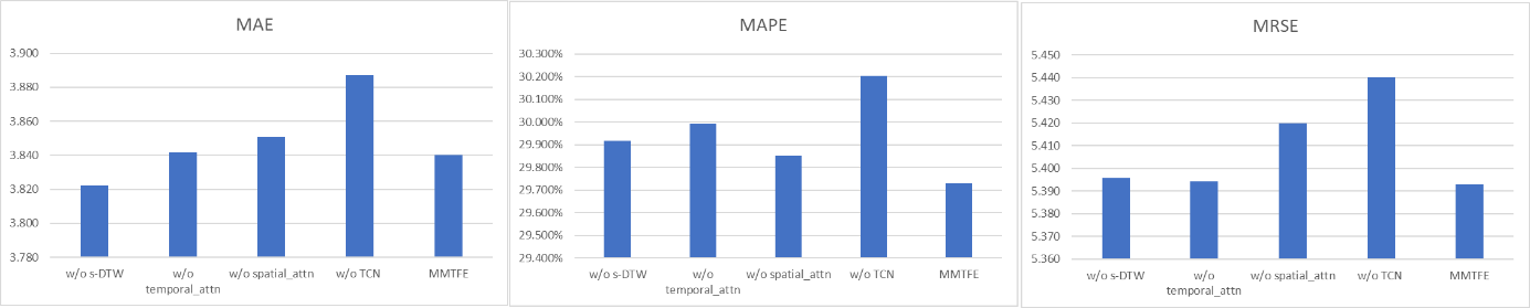
Figure 1. Ablation study on CHBike dataset.

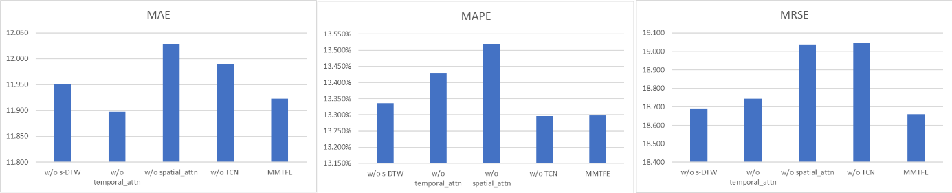
Figure 2. Ablation study on NYTaxi dataset.

As shown in Figure 1 and Figure 2, these two figures illustrate the performance outcomes of these variants on CHBike and NYTaxi. The results indicate that (1) soft DTW performs better than DTW in the majority of cases, (2) the performance of the variant MMTFE without Temporary Attention has been significantly enhanced on several datasets, thereby underscoring its value, and (3) the performance of the variant MMTFE without TCN has been significantly enhanced on several datasets, thereby indicating that time dependence is a pivotal element to be taken into account in the model.

6. Conclusions

This research proposes a hybrid transformer-TCN model for traffic prediction, exhibiting strong dynamic spatiotemporal dependence. We introduce a Multi-Modal traffic encoder comprising temporal attention, spatial attention, and temporal convolutional network components. These elements collectively capture short-term and long-term temporal and spatial dependencies. We validated our model's effectiveness through experiments on two real-world datasets. Future research will explore the application of large language models to traffic prediction tasks [22], aiming to improve the efficiency and performance of traffic forecasting systems.

References

[1]. Tedjopurnomo, D. A., Bao, Z., Zheng, B., Choudhury, F. M., & Qin, A. K. (2020). A survey on modern deep neural network for traffic prediction: Trends, methods and challenges. IEEE Transactions on Knowledge and Data Engineering, 34(4), 1544-1561.
[2]. Yin, X., Wu, G., Wei, J., Shen, Y., Qi, H., & Yin, B. (2021). Deep learning on traffic prediction: Methods, analysis, and future directions. IEEE Transactions on Intelligent Transportation Systems, 23(6), 4927-4943.
[3]. Duan, Y., Yisheng, L. V., & Wang, F. Y. (2016). Travel time prediction with LSTM neural network. In 2016 IEEE 19th international conference on intelligent transportation systems (ITSC), 1053-1058.
[4]. Zhang, J., Zheng, Y., & Qi, D. (2017). Deep spatio-temporal residual networks for citywide crowd flows prediction. In Proceedings of the AAAI conference on artificial intelligence, 31(1).
[5]. Yao, H., Wu, F., Ke, J., Tang, X., Jia, Y., Lu, S., ... & Li, Z. (2018). Deep multi-view spatial-temporal network for taxi demand prediction. In Proceedings of the AAAI conference on artificial intelligence, 32(1).
[6]. Li, Y., Yu, R., Shahabi, C., & Liu, Y. (2017). Diffusion convolutional recurrent neural network: Data-driven traffic forecasting. arXiv preprint arXiv:1707.01926.
[7]. Yu, B., Yin, H., & Zhu, Z. (2017). Spatio-temporal graph convolutional networks: A deep learning framework for traffic forecasting. arXiv preprint arXiv:1709.04875.
[8]. Wu, Z., Pan, S., Long, G., Jiang, J., & Zhang, C. (2019). Graph wavenet for deep spatial-temporal graph modeling. arXiv preprint arXiv:1906.00121.
[9]. Guo, S., Lin, Y., Feng, N., Song, C., & Wan, H. (2019). Attention based spatial-temporal graph convolutional networks for traffic flow forecasting. In Proceedings of the AAAI conference on artificial intelligence, 33(01), 922-929.
[10]. Zheng, C., Fan, X., Wang, C., & Qi, J. (2020). Gman: A graph multi-attention network for traffic prediction. In Proceedings of the AAAI conference on artificial intelligence, 34(01), 1234-1241.
[11]. Bai, L., Yao, L., Li, C., Wang, X., & Wang, C. (2020). Adaptive graph convolutional recurrent network for traffic forecasting. Advances in neural information processing systems, 33, 17804-17815.
[12]. Cui, Z. (2021). Deep Learning for Short-Term Network-Wide Road Traffic Forecasting. University of Washington.
[13]. Chen, W., Chen, L., Xie, Y., Cao, W., Gao, Y., & Feng, X. (2020). Multi-range attentive bicomponent graph convolutional network for traffic forecasting. In Proceedings of the AAAI conference on artificial intelligence, 34(04), 3529-3536.
[14]. Jiang, J., Han, C., Zhao, W. X., & Wang, J. (2023). Pdformer: Propagation delay-aware dynamic long-range transformer for traffic flow prediction. In Proceedings of the AAAI conference on artificial intelligence, 37(4), 4365-4373.
[15]. Loshchilov, I., & Hutter, F. (2017). Fixing weight decay regularization in adam. arXiv preprint arXiv:1711.05101, 5.
[16]. Liu, C., Yang, S., Xu, Q., Li, Z., Long, C., Li, Z., & Zhao, R. (2024). Spatial-temporal large language model for traffic prediction. arXiv preprint arXiv:2401.10134.
[17]. Wu, Z., Pan, S., Long, G., Jiang, J., Chang, X., & Zhang, C. (2020). Connecting the dots: Multivariate time series forecasting with graph neural networks. In Proceedings of the 26th ACM SIGKDD international conference on knowledge discovery & data mining, 2020, 753-763.
[18]. Li, M., & Zhu, Z. (2021). Spatial-temporal fusion graph neural networks for traffic flow forecasting. In Proceedings of the AAAI conference on artificial intelligence, 35(5), 4189-4196.
[19]. Choi, J., Choi, H., Hwang, J., & Park, N. (2022). Graph neural controlled differential equations for traffic forecasting. In Proceedings of the AAAI conference on artificial intelligence, 36(6), 6367-6374.
[20]. Zheng, C., Fan, X., Wang, C., & Qi, J. (2020). Gman: A graph multi-attention network for traffic prediction. In Proceedings of the AAAI conference on artificial intelligence, 34(01), 1234-1241.
[21]. Guo, S., Lin, Y., Wan, H., Li, X., & Cong, G. (2021). Learning dynamics and heterogeneity of spatial-temporal graph data for traffic forecasting. IEEE Transactions on Knowledge and Data Engineering, 34(11), 5415-5428.
[22]. Cuturi, M., & Blondel, M. (2017). Soft-dtw: a differentiable loss function for time-series. In International conference on machine learning. PMLR, 2017, 894-903.
Cite this article
Liang,B. (2024). Traffic Flow Prediction with Strong Dynamic Spatiotemporal Dependence Using a Hybrid Model of Transformer and TCN. Applied and Computational Engineering,111,45-53.
Data availability
The datasets used and/or analyzed during the current study will be available from the authors upon reasonable request.
Disclaimer/Publisher's Note
The statements, opinions and data contained in all publications are solely those of the individual author(s) and contributor(s) and not of EWA Publishing and/or the editor(s). EWA Publishing and/or the editor(s) disclaim responsibility for any injury to people or property resulting from any ideas, methods, instructions or products referred to in the content.
About volume
Volume title: Proceedings of CONF-MLA 2024 Workshop: Mastering the Art of GANs: Unleashing Creativity with Generative Adversarial Networks
© 2024 by the author(s). Licensee EWA Publishing, Oxford, UK. This article is an open access article distributed under the terms and
conditions of the Creative Commons Attribution (CC BY) license. Authors who
publish this series agree to the following terms:
1. Authors retain copyright and grant the series right of first publication with the work simultaneously licensed under a Creative Commons
Attribution License that allows others to share the work with an acknowledgment of the work's authorship and initial publication in this
series.
2. Authors are able to enter into separate, additional contractual arrangements for the non-exclusive distribution of the series's published
version of the work (e.g., post it to an institutional repository or publish it in a book), with an acknowledgment of its initial
publication in this series.
3. Authors are permitted and encouraged to post their work online (e.g., in institutional repositories or on their website) prior to and
during the submission process, as it can lead to productive exchanges, as well as earlier and greater citation of published work (See
Open access policy for details).