1. Introduction

Convolutional Neural Networks (CNNs) are feedforward neural networks tailored for processing two-dimensional data, particularly images, exhibiting remarkable capabilities in image and speech recognition. Since the concept of "receptive field" was introduced by Hubel and Wiesel in 1962, CNNs have evolved significantly, beginning with Fukushima Kunihiko's "Neocognitron" in 1980 and further advancing with LeNet-5 in 1998, which laid the groundwork for modern architectures. The breakthrough came in 2012 when Hinton's AlexNet substantially reduced the error rate in the ImageNet competition, leading to the emergence of models like GoogLeNet and DenseNet that have enhanced performance. Despite these advancements, challenges remain, including the transition from supervised to unsupervised learning, optimization of neural network efficiency and accuracy, robustness against adversarial samples, and GPU resource limitations, indicating notable research gaps. This study examines the optimization of CNN efficiency and accuracy through hyperparameter tuning, specifically focusing on influential factors such as learning rate, dropout rate, batch size, and epoch number, and their effects on a simple CNN model trained on the CIFAR-10 dataset. The research employs data analysis and model comparison to identify how these hyperparameters influence model performance. The findings aim to address current challenges in CNNs, particularly in enhancing performance in unsupervised learning and improving robustness against adversarial samples. While the simple CNN model serves as a foundational analysis, it is anticipated that the insights gained will guide further explorations into optimizing complex architectures like AlexNet, contributing to the future development of CNNs in diverse applications.

2. Experiment

2.1. The CIFAR-10 dataset preparing

Before initiating the actual training runs, it is essential to establish the dataset and set some fixed parameters.High-quality images significantly enhance object recognition or classification rates compared to unprocessed, noisy images[1]. For our project, we selected the "CIFAR-10 Dataset," which is a benchmark dataset commonly used in image classification tasks. The CIFAR-10 dataset comprises 60,000 color images, each with dimensions of 32x32 pixels. These images are divided into 10 distinct classes, with each class containing 6,000 images. The dataset is split into 50,000 images for training and 10,000 images for testing. This distribution ensures that the model is trained on a large portion of the data while reserving a substantial set of images for evaluation.To achieve a robust evaluation of the model’s performance, we allocate 80% of the datasets to the training set and 20% to the test set.

2.2. The architecture of convolutional neural networks(CNNs)

To ensure consistency and reproducibility in the partitioning of the dataset, we can use the parameter "random_state=42" as the seed for the random number generator. This parameter ensures consistent results across multiple runs by maintaining the same data split every time the code executes. Regarding the model structure, it is designed to handle the specific requirements of image classification tasks. LeCun, the originator of convolutional neural networks, proposed LeNet in 1998 to solve the visual task of handwritten digit recognition. Since then, the most basic architecture of CNN has been settled: convolutional layer, pooling layer, and fully connected layer[2]. The architecture includes several key components: the input layer, convolutional layers, pooling layers, fully connected layers, dropout layers, and the output layer. VGG Net highlights the importance of depth in convolutional networks, suggesting that a CNN should maintain a deep yet straightforward structure to effectively capture the hierarchical processing of visual data[3]. The fixed image size facilitates processing, and the dataset image itself is 32x32 pixels, so the input layer is designed to process color images with input shapes of (32,32,3). This shape represents images of 32x32 pixels, with 3 color channels corresponding to the RGB values. This allows the model to process and analyze the color information present in the images.Convolutional Layers: The convolutional part of the network consists of six layers organized sequentially. The first convolutional layer applies 32 convolutional kernels of size 3x3. These kernels scan the image to detect various features. The second convolutional layer uses 64 kernels of size 3x3, which allows the model to learn more complex features. The third convolutional layer employs 128 kernels of size 3x3, further enabling the model to capture intricate patterns and details in the images. The Rectified Linear Unit (ReLU) activation function is used in each convolutional layer. This gives the model nonlinearity and helps it learn complex patterns. A pooling layer follows each convolutional layer. The pooling layers use a 2x2 pooling kernel to downsample the feature maps. This downsampling reduces the spatial dimensions of the feature maps while retaining important information. Pooling helps reduce the computational load and mitigates the risk of overfitting by abstracting the feature maps. Fully Connected Layers: After the convolutional and pooling layers, the model transitions to the fully connected layers. The fully connected layer flattens the high-level features extracted by the convolutional layers and connects them to a dense layer with 128 neurons. This layer uses the ReLU activation function to introduce further non-linearity and enhance the model’s ability to learn complex representations. Dropout Layers: The incorporation of dropout layers prevents overfitting by randomly setting a fraction of input units to zero at each update during training. This helps to reduce neuron co-adaptations and promotes network sparsity. Output Layer: The final layer is the output layer, which consists of 10 neurons, corresponding to the 10 categories in the CIFAR-10 dataset. This layer uses the softmax activation function to produce a probability distribution over the 10 classes. The softmax function converts the raw output scores into probabilities, which facilitates the classification of images into one of the 10 categories. The choice of these layers and their configurations is pivotal in determining the model's performance. The convolutional layers are crucial for feature extraction, while the pooling layers help in reducing computational complexity and mitigating overfitting. The fully connected layers, along with dropout, are essential for learning complex representations and enhancing generalization. The output layer's softmax function is crucial for generating class probabilities and making final predictions.

In summary, the CIFAR-10 dataset, combined with our meticulously designed CNN architecture, serves as the foundation for our image feature extraction project. By leveraging this structure, we aim to optimize model performance and achieve accurate and reliable feature extraction results.

3. Analysis and Discussion

In my experimentation, the primary parameters adjusted were the learning rate and dropout rate, with the epoch number set to 50 and the batch size at 64. The selection of the optimal learning rate is crucial, as it significantly influences whether the neural network can converge to the global minimum. Setting the learning rate too high tends to skip over the global minimum, causing the network to oscillate around it without ever truly converging to it. Conversely, a smaller learning rate facilitates convergence to the global minimum, but it takes more time to do so. Thus, while a higher learning rate can expedite the convergence process, it may lead to unstable training results. On the other hand, a lower learning rate, while promoting stability, may slow down convergence and increase the risk of the model getting stuck in a local minimum. Increasing the learning rate can improve results faster, but it may also cause the model to oscillate around the best solution or diverge[4]. On the other hand, decreasing the learning rate can lead to more stable model convergence, but it may slow down the training process and increase the risk of getting stuck in local optima[5]. Furthermore, dynamic learning rate adjustment methods, such as learning rate decay, have been demonstrated to greatly improve model performance[6]. However, dynamically modifying the learning rate may also increase computational costs[7]. The dropout rate is another critical parameter that helps prevent overfitting, enhances the model’s generalization capability, promotes network sparsity, and reduces co-adaptability among neurons. Nevertheless, excessively high dropout rates may introduce the risk of underfitting. Using "dropout," a technique where each hidden neuron's output is set to zero with a probability of 0.5, efficiently reduces test errors in large neural networks without significantly increasing training costs. Therefore, it is essential to test learning rates and dropout rates independently by controlling other variables. An appropriate dropout rate can effectively prevent overfitting and improve the model’s performance on new data [8]. Research indicates that higher dropout rates can significantly reduce overfitting but may also make the model training more challenging[9]. Conversely, a lower dropout rate affects the model’s structure less but might not be as effective in preventing overfitting[10].Practically, we can evaluate the learning rate using the following parameters: [0.01, 0.001, 0.0001], and assess the dropout rate using values of [0.3, 0.5, 0.7]. By plotting accuracy and loss curves for these variables, it is theoretically possible to pinpoint the optimal learning rate. When the learning rate is set to 0.01, the model tends to underfit, as evidenced by the non-linear relationship between training accuracy, test accuracy, training loss rate, and test loss rate. Figures 1, 2, and 3 show the accuracy and loss curves obtained when the learning rate is set to 0.01.

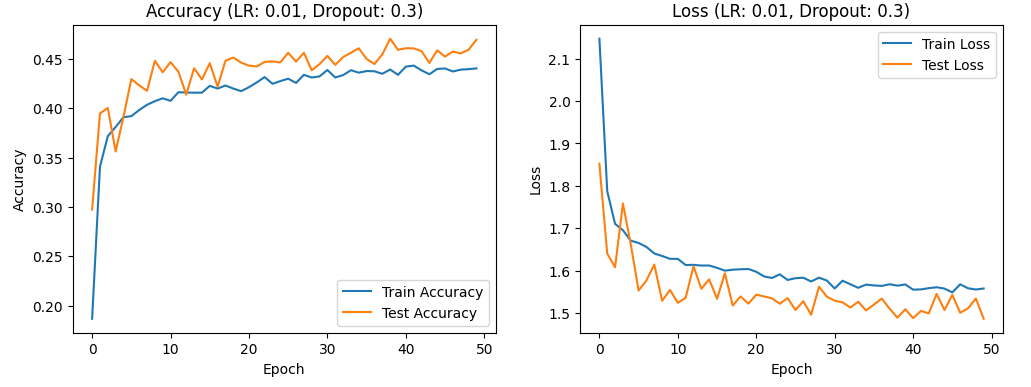
Figure 1. the curve of accuracy and loss(LR:0.01,Dropout:0.3)

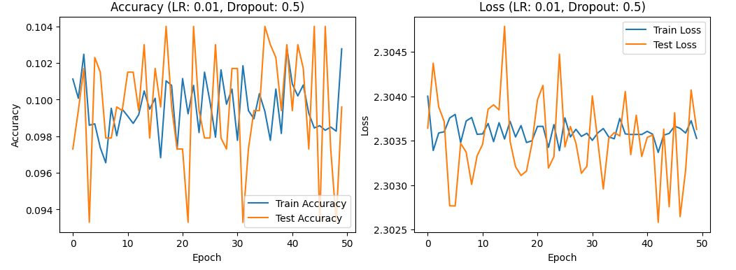
Figure 2. the curve of accuracy and loss(LR:0.01,Dropout:0.5).

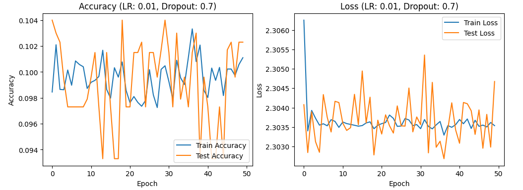
Figure 3. the curve of accuracy and loss(LR:0.01,Dropout:0.7).

With a learning rate of 0.001, there is a gradual increase in both test and training accuracy, initially rapid then slower, while the test and training loss rates decrease and then increase. This suggests that the learning rate is still too high, which could lead to overfitting and necessitate further reduction. Figures 4, 5, and 6 show the accuracy and loss curves obtained when the learning rate is set to 0.001.

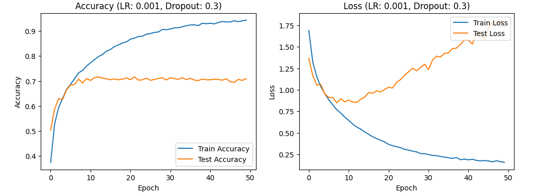
Figure 4. the curve of accuracy and loss(LR:0.001,Dropout:0.3).

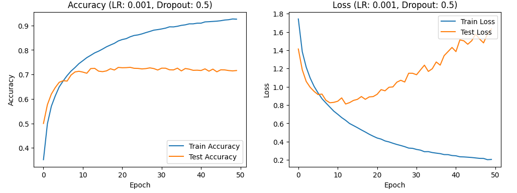
Figure 5. the curve of accuracy and loss(LR:0.001,Dropout:0.5).

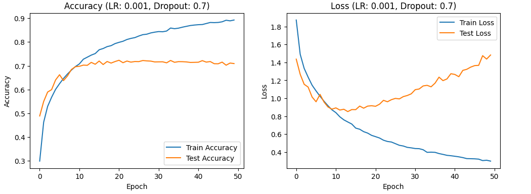
Figure 6. the curve of accuracy and loss(LR:0.001,Dropout:0.7).

At a learning rate of 0.0001, both training accuracy and test accuracy exhibit a trend of initially rapid improvement followed by a slower increase. Figures 7, 8, and 9 show the accuracy and loss curves obtained when the learning rate is set to 0.0001.

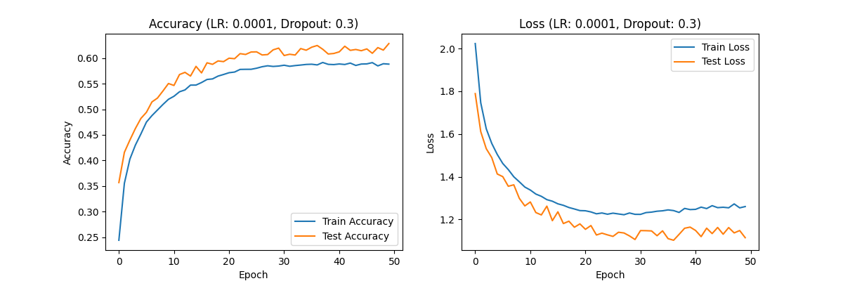
Figure 7. the curve of accuracy and loss(LR:0.0001,Dropout:0.3).

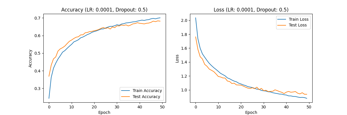
Figure 8. the curve of accuracy and loss(LR:0.0001,Dropout:0.5).

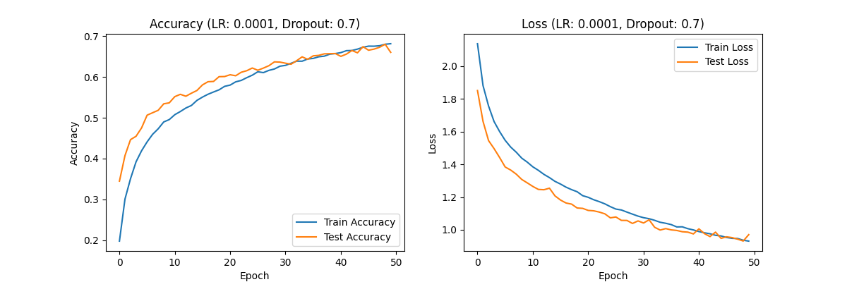
Figure 9. the curve of accuracy and loss(LR:0.0001,Dropout:0.7).

Similarly, the training and test loss rates show a decreasing trend, first rapid and then gradual, with the overall curve appearing relatively smooth. This suggests that a learning rate of 0.0001 is more appropriate, as it avoids overfitting and underfitting issues and provides better training results. When evaluating dropout rates with the optimal learning rate of 0.0001, the results across different dropout settings exhibit similar trends. The training and test accuracies show an initial rapid increase followed by a slower growth, while the training and test loss rates exhibit a decreasing trend initially rapid and then slow.

Observe the previously provided curves for learning rate 0.0001 with dropout rates of 0.3, 0.5, and 0.7, shown in Figures 7, 8, and 9, respectively. Since changes in dropout rate do not intuitively affect overall optimization levels, it suggests that under the optimal learning rate, varying dropout rates have a less pronounced impact on model performance. The curve appears smoothest with a dropout rate of 0.5, indicating that the model performs best with this dropout rate when using a learning rate of 0.0001.

The batch size and the number of epochs are the hyperparameters under adjustment in the current analysis. After setting the group's hyperparameters, which include a learning rate of 0.0001 and a dropout rate of 0.5, the focus shifts to fine-tuning these specific parameters. Epochs represent the number of complete passes through the training dataset. If the dataset is used E times during training, the model is said to have undergone E epochs. The number of epochs significantly influences the model's training duration, accuracy, potential overfitting, convergence speed, and the consumption of computational resources. The number of epochs is a crucial hyperparameter that influences the training duration and the risk of overfitting. Early stopping is commonly used to prevent overfitting by halting training when performance on a validation set starts to degrade[11].Increasing the number of epochs generally leads to better performance on the training data, but if not monitored carefully, it may lead to overfitting where the model performs poorly on unseen data"[12]. Excessive epochs can lead to overfitting and inefficient use of resources, while too few epochs may result in underfitting and suboptimal model performance. At the current stage, the batch size remains fixed at 64.

With an epoch count of 10, the program completes the training in approximately 15 minutes. During this period, both the training accuracy and test accuracy show an increasing trend, initially rapid and then slower. Specifically, the training accuracy fluctuates between 0.35 and 0.75, while the test accuracy ranges from 0.50 to 0.70. Conversely, the loss rate decreases over time, first rapidly and then more gradually. The training loss rate ranges from 0 to 1.8, and the test loss rate spans from 0.8 to 1.4.Figure 10 shows the image results.

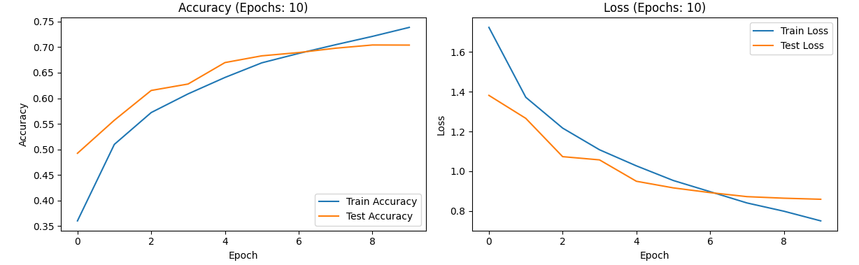
Figure 10. the curve of accuracy and loss(the number of epochs:10).

With the epoch count increased to 50, the training duration extends to about one hour and forty minutes. Initially, before reaching epoch 10, both the training and test accuracies rise steadily, although the rate of increase slows down over time. After epoch 10, the test accuracy fluctuates around 0.7, while the training accuracy continues to increase, reaching up to 0.9. The loss rates exhibit a different pattern compared to epoch 10; the training loss rate decreases from 1.8 to approximately 0.2, approaching zero. However, the test loss rate decreases initially but starts to rise after epoch 10, peaking at around 1.4 before epoch 40 and then increasing further. This indicates overfitting beyond epoch 10, suggesting that an optimal epoch setting would be around 10. Figure 10 shows the image results.Given that training time can be lengthy and overfitting becomes evident with higher epochs, testing with 100 epochs may not be necessary.

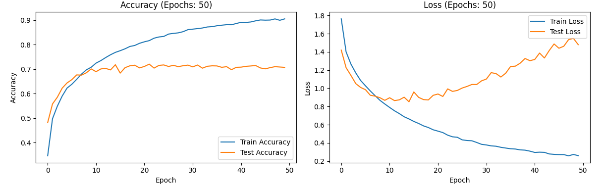
Figure 11. the curve of accuracy and loss(the number of epochs:50).

The impact of batch size on the model manifests in aspects such as training stability, training speed, model generalization, memory usage, and the effectiveness of the optimizer. Larger batch sizes generally improve training speed but may lead to less stable generalization compared to smaller batch sizes, which often offer better generalization performance[13]. The batch size choice has an impact on training stability and speed. Smaller batch sizes tend to provide more accurate estimates of the gradient but require more iterations to converge"[14]. Smaller batch sizes often enhance generalization but result in slower training, while larger batch sizes can accelerate training but may reduce generalization and increase memory demands. Testing with batch sizes of 32, 64, and 128 at an optimal epoch count of 10 reveals similar trends across the three data sets. Specifically, training and test accuracy show an increasing trend, initially rapid and then slowing, while training and test loss rates exhibit a decreasing trend, first rapidly and then more slowly.

Comparing the results: For a batch size of 32: Training accuracy ranges from 0.35 to 0.75, test accuracy from 0.50 to 0.70, training loss rate from 0.6 to 1.7, and test loss rate from 0.8 to 1.4.Figure 12 shows the image results.

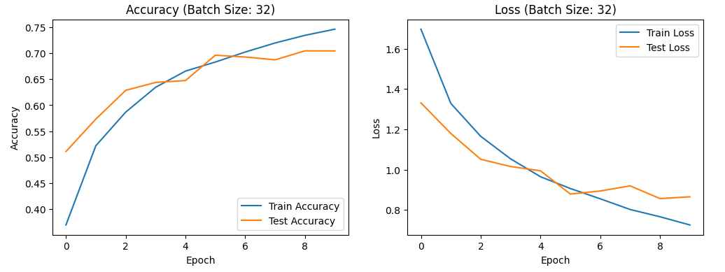
Figure 12. the curve of accuracy and loss(batch size:32).

For a batch size of 64: training accuracy ranges from 0.35 to 0.70, test accuracy from 0.45 to 0.70, training loss rate from 0.8 to 1.8, and test loss rate from 0.8 to 1.6.Figure 13 shows the image results.

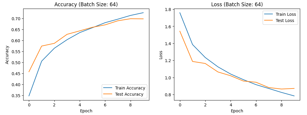
Figure 13. the curve of accuracy and loss(batch size:64).

For a batch size of 128: training accuracy ranges from 0.30 to 0.70, test accuracy from 0.45 to 0.70, training loss rate from 0.8 to 1.9, and test loss rate from 0.8 to 1.5.Figure 14 shows the image results.

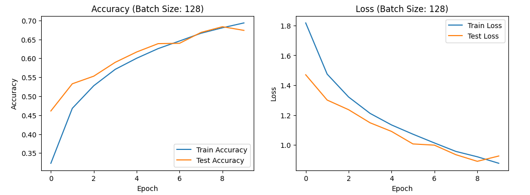
Figure 14. the curve of accuracy and loss(batch size:128).

Overall, variations in batch size result in only slight changes in accuracy and loss rates. This suggests that batch size has a minor effect on the model's overall optimization, though a batch size of 32 might offer a slight improvement. Moreover, batch normalization can mitigate some of the challenges associated with varying batch sizes, including those related to gradient stability and model generalization" [15]. Interestingly, setting the epoch count to 10 appears to be insufficient, suggesting the need to increase the dataset size for practical applications.

4. Conclusion

In general, our group's project centers on the topic of "image feature extraction using convolutional neural networks (CNNs)." During the course of this project, we explored a range of hyperparameters that influence the optimization of CNNs, ultimately narrowing our focus to the learning rate and dropout rate. Based on our findings, I conducted additional tests to assess the impact of batch size and epoch number, using the group's data as a reference. Utilizing the CIFAR-10 dataset, we methodically determined the optimal learning rate and dropout rate. We rigorously analyzed how these hyperparameters affect various performance metrics of the model, including training accuracy, test accuracy, training loss rate, and test loss rate across different settings. Our experiments consistently demonstrated that the model achieves its best performance with a learning rate set to 0.0001 and a dropout rate of 0.5. In addition to these findings, I observed that batch size had a relatively minor impact on overall model optimization. However, a slight improvement was noted when the batch size was set to 32. Furthermore, as the number of epochs increased, the model showed a tendency toward overfitting. To mitigate this, I recommend setting the number of epochs to 10, as this balance helps avoid overtraining while also conserving computational resources. It is important to note that setting the epoch number too low can result in insufficient training passes, which might hinder a thorough analysis of other hyperparameters. Therefore, adjusting the epoch number according to the specific requirements of the dataset and model is crucial. Through these strategic adjustments, we have successfully optimized the model's performance, achieving a more effective feature extraction capability.

References

[1]. Amir Ghasem, Nasrin Bayat, Fatemeh Mottaghian & Akram Bayat (2023). Improving Performance of Object Detection Using the Mechanisms of Visual Recognition in Humans. arXiv preprint, 2301.09667.Retrieved from https://doi.org/10.48550/arXiv.2301.09667
[2]. Siqi Lv, Wangli He, Feng Qian&Jinde Cao(2018). Leaderless synchronization of coupled neural networks with the event-triggered mechanism. Neural Networks, 105, 316-327.Retrieved from https://doi.org/10.1016/j.neunet.2018.05.012
[3]. Simonyan, K., & Zisserman, A. (2015). Very Deep Convolutional Networks for Large-Scale Image Recognition. International Conference on Learning Representations (ICLR). Retrieved from https://doi.org/10.48550/arXiv.1409.1556.
[4]. Y. Bengio, P. Simard, & P. Frasconi (1994). "Learning Long-Term Dependencies with Gradient Descent is Difficult." IEEE Transactions on Neural Networks, 5(2), 157-166.Retrieved from https://ieeexplore.ieee.org/document/279181
[5]. Loshchilov, I., & Hutter, F. (2017). "SGDR: Stochastic Gradient Descent with Warm Restarts." In Proceedings of the International Conference on Learning Representations (ICLR). Retrieved from https://doi.org/10.48550/arXiv.1608.03983
[6]. Kaichao You, Mingsheng Long, Jianmin Wang, & Michael I. Jordan.(2019). How Does Learning Rate Decay Help Modern Neural Networks?
[7]. Smith, L. N. (2017). Cyclical Learning Rates for Training Neural Networks. In Proceedings of the IEEE Conference on Computer Vision and Pattern Recognition (CVPR) (pp. 184-190). https://ieeexplore.ieee.org/abstract/document/7926641
[8]. Srivastava, N., Hinton, G. E., Krizhevsky, A., Sutskever, I., & Salakhutdinov, R. (2014). Dropout: A technique to prevent overfitting in neural networks. Journal of Machine Learning Research, 15, 1929-1958. http://www.jmlr.org/papers/volume15/srivastava14a/srivastava14a.pdf
[9]. Zhang, Y. (2018). Impact of dropout rates on overfitting and model training. International Journal of Machine Learning and Computing, 8(5), 478-484. https://doi.org/10.18178/ijmlc.2018.8.5.686
[10]. Li, Q., & Ke, W. (2024). Investigating the Synergistic Effects of Dropout and Residual Connections on Language Model Training. https://arxiv.org/pdf/2410.01019
[11]. Srivastava, N., Hinton, G., Krizhevsky, A., Sutskever, I., & Salakhutdinov, R. (2014). Dropout: A simple way to prevent neural networks from overfitting. *Journal of Machine Learning Research,15*,1929-1958.https://www.jmlr.org/papers/volume15/srivastava14a/srivastava14a.pdf
[12]. Ajayi, O. G., & Ashi, J. (2023). Effect of varying training epochs of a Faster Region-Based Convolutional Neural Network on the Accuracy of an Automatic Weed Classification Scheme. Smart Agricultural Technology, 3, 100128. https://www.sciencedirect.com/science/article/pii/S2772375522000934
[13]. Keskar, N. S., Mudigere, D., Nocedal, J., Smelyanskiy, M., & Tang, P. T. P. (2016). On Large-Batch Training for Deep Learning: Generalization Gap and Sharp Minima. arXiv preprint arXiv:1609.04836. https://arxiv.org/abs/1609.04836
[14]. Wilson, D. R., & Martinez, T. R. (2003). The general inefficiency of batch training for gradient descent learning. Neural Networks, 16(10), 1429-1451. https://www.sciencedirect.com/science/article/abs/pii/S0893608003001382?via%3Dihub
[15]. Santurkar, S., Tsipras, D., Ilyas, A., & Madry, A. (2019). “How Does Batch Normalization Help Optimization?” arXiv preprint arXiv: 1805.11604. Retrieved from https://arxiv.org/abs/1805.11604
Cite this article
Xiang,S. (2024). Research on Image Feature Extraction Based on Convolutional Neural Network. Applied and Computational Engineering,107,24-33.
Data availability
The datasets used and/or analyzed during the current study will be available from the authors upon reasonable request.
Disclaimer/Publisher's Note
The statements, opinions and data contained in all publications are solely those of the individual author(s) and contributor(s) and not of EWA Publishing and/or the editor(s). EWA Publishing and/or the editor(s) disclaim responsibility for any injury to people or property resulting from any ideas, methods, instructions or products referred to in the content.
About volume
Volume title: Proceedings of the 2nd International Conference on Machine Learning and Automation
© 2024 by the author(s). Licensee EWA Publishing, Oxford, UK. This article is an open access article distributed under the terms and
conditions of the Creative Commons Attribution (CC BY) license. Authors who
publish this series agree to the following terms:
1. Authors retain copyright and grant the series right of first publication with the work simultaneously licensed under a Creative Commons
Attribution License that allows others to share the work with an acknowledgment of the work's authorship and initial publication in this
series.
2. Authors are able to enter into separate, additional contractual arrangements for the non-exclusive distribution of the series's published
version of the work (e.g., post it to an institutional repository or publish it in a book), with an acknowledgment of its initial
publication in this series.
3. Authors are permitted and encouraged to post their work online (e.g., in institutional repositories or on their website) prior to and
during the submission process, as it can lead to productive exchanges, as well as earlier and greater citation of published work (See
Open access policy for details).