1. Introduction

Since 1880, the Earth’s temperature has increased at a pace of 0.14° Fahrenheit (0.08° Celsius) every decade; the rate of warming since 1981 is even more than double that, at 0.32 °F (0.18 °C) per decade. 2023 was the warmest year in modern temperature records, and global temperatures are still rising [1]. Warmer temperatures can lead to a chain reaction of other global changes [2]. Therefore, the urgency for understanding and predicting environmental changes has never been more crucial. Environmental factors, such as global temperature greenhouse gas emissions, lead to the effects of global warming and its cascading effects on the environment, human health, and the economy. The ability to predict these specific factors will lead to a future where we can create strategies to adapt to and mitigate the effects of these inevitable changes and serve as a crucial reminder of our crisis. Whether through green energy, political intervention through carbon taxation, or reforestation, knowing where we currently stand and where we are going is an excellent place to start [3].

As a natural child of sequence and visual data, many tools have been used to predict time series data, specifically temperature data. We can categorize these into three main groups: 1) Non-Machine-Learning (i.e., statistic-based) approaches, 2) Recurrent Neutral Network / Long-Short Term Memory approaches, and 3) Transformer-based Models.

Traditional statistic-based algorithms have been the cornerstone of climate forecasting. Methods such as the AutoRegressive Integrated Moving Average (ARIMA), proposed by Box et al. in 2015, is a stochastic model that uses autoregression, differencing, and moving average components to capture temporal patterns in time series data [4]. This method was applied to environmental prediction through temperature forecasting in 2013 by Ye et al. [5]. The Seasonal and Trend Decomposition of Time Series with Loess (STL) is a standard deterministic method used for time series forecasting; with Loess (locally estimated scatterplot smoothing), the process extracts trends and seasonal components from time series data [6]. Cleveland et al. in 1990 have used STL to predict CO \( {​_{2}} \) emissions.

As the complexities of environmental data and the demand for more accurate predictions grew, the focus shifted towards more advanced models capable of capturing the deeper temporal intricacies of time series data. This led to the development of Recurrent Neural Network (RNN) based models, such as the Long-Short Term Memory (LSTM) approach. In 1997, Hochreiter et al. proposed that LSTMs were designed to enhance RNN’s internal memory mechanism and its performance to model long-term dependencies [7]. They have been widely used in climate forecasting, demonstrating their ability to model complex environmental phenomena. In 2022 Hunt et al. used LSTMs to enhance river streamflow forecasts, highlighting their superiority over traditional physics-based models [8]. Similarly in 2022, El-Habil and Abu-Naser leveraged a convolutional LSTM model for global temperature forecasting, achieving high testing accuracy and demonstrating the potential of LSTMs in handling intricate climate patterns [9].

Recently, the transformer and specialized time series prediction models have emerged. The transformer, introduced by Vaswani et al. in 2017, introduced a novel approach to predicting sequenced data. The encoder/decoder-based model was mainly used in natural language processing, image recognition, and other text-based purposes [10]. The attention mechanism introduced allows the model to recognize the importance of different tokens in a sequence without preprocessing. In 2022 Alerskans et al. utilized transformers for climate forecasting and global temperature prediction [11]. Adaptations of the transformer model have also been used to predict other time series data, such as the Informer introduced by Zhou et al. proposed in 2021, specifically designed for environmental forecasting. They intended to improve the transformer architecture to be computationally efficient while maintaining high prediction accuracy [12].

In this study, I explore the potential of a customized transformer model inspired by the work of "Attention is All You Need" [10] to enhance time series prediction. Focusing on environmental data such as global temperature and greenhouse gas emissions, this project leverages the attention mechanism to understand the sequence data better, allowing the model to outperform existing models in accuracy and efficiency.

2. Problem Formulation

Assume we have a sequence of temperature data \( x \) collected at a successive time window \( T \) . We denote \( {x_{0}} \) as the current data point ( \( T=0 \) ) and correspondingly represent the rest of the data as \( {x_{+i}} \) the \( i \) -th future time step, or \( {x_{-i}} \) , the \( i \) -th previous data point. This project aims to try to generate a model that can take in \( {x_{-i}} \) and \( {x_{0}} \) and predict \( {x_{+i}} \) , predicting the future temperature changes based on current status and historical observations.

There are two ways to achieve this goal: 1) a single-step prediction task and 2) a multiple-step prediction task. A single-step prediction aims to forecast the immediate next value of the sequence, denoted as \( {x_{+1}} \) , utilizing a range of values, including the current value, \( {x_{0}} \) , and a set of precedenting values, \( {x_{-1}},{x_{-2}},… \) . Multi-step prediction aims to predict several future values altogether, denoted by \( {x_{+1}},{x_{+2}},… \) , which can either be done through a single, comprehensive model output or iteratively, where the model’s immediate outputs are recursively used as the new inputs for the next prediction. In this project, I focus on the multi-step prediction formulation, which can be categorized again into two types: single-shot and autoregressive models.

2.1. Single-Shot Formulation

Figure 1. Single-Shot vs. Autoregressive Prediction Process.

In single-shot formulation, the model is trained to output the entire sequence of future values simultaneously. This method eliminates the dependencies between predictions in the sequence and reduces the possibility of cumulative errors common in recursive prediction processes. This is most suitable for situations where a full forecast is needed, and the future data points lack interdependencies among each other. However, a notable limitation of this approach is its inflexibility regarding changes to the forecast horizon. If the desired prediction timeframe changes, the model must be retrained to fit the new output structure since it cannot be adjusted to adapt to different forecasting horizons. This means carefully considering the forecast period during the model design is necessary.

2.2. Autoregressive Formulation

In an autoregressive prediction, the model sequentially makes predictions for future values using its preceding predictions as the inputs. The model makes multiple, single-step predictions and then shifts its input sequence to include that new singular prediction point. This model shines when the predicted data is highly interdependent or when the forecast horizon is extended. This recursive strategy also introduces flexibility and adaptability to the forecast horizons. However, it comes with its drawbacks. The self-referencing nature of the model carries the risk of error propagation. Since each prediction relies on the accuracy of the previous predictions, any initial prediction errors can be magnified through the forecast horizon.

2.3. Loss Function Design

The choice of the loss function and optimizer is similar for each formulation. Since our problem fits a typical regression problem, a Mean Squared Error (MSE) loss is appropriate, penalizing significant errors and encouraging model accuracy. For the single-shot formulation, the loss is calculated and backpropagated after every forward calculation, minimizing the error across the entire output sequence at once. For the autoregressive approach, the predictions are made sequentially, and the loss is computed after generating the sequence as a whole; this allows the model to evaluate its performance over the entire forecast horizon while adjusting each iterative calculation.

3. Model Structure

3.1. Multi-Task Learning

Since many other environmental factors are related to temperature changes, I experimented with a multi-task learning framework. The motivation is that multiple tasks can usually help the prediction accuracy of the individual task. This process involves predicting the global temperature anomaly and the emission of greenhouse gasses, which naturally have some correlations. Both tasks will be predicted simultaneously and aggregated to contribute to the loss. This way, the model can balance the importance of each task individually during training and correct both tasks simultaneously, leading to a steadier and more accurate prediction.

3.2. Features

Monthly global temperature data will be inputted into the model for single-task prediction. The data has been segmented into consistent sequences for training and evaluation purposes. Each data point contains information on thirteen location ranges and is represented as a tensor of dimension thirteen. This project specifically focuses on the temperature anomaly present in the dataset and will use that as the main feature for prediction.

For the multi-task prediction, the input to the model will be the annual greenhouse gas emission and global temperature data. For this, I aggregated the global temperature data to an annual scale to match the temporal resolution of the greenhouse gas emissions data. Since the greenhouse emission data does not contain multiple locations, a padding process must match its dimensions with the global temperature data. The two tensors of equivalent dimensions are concatenated and passed through the model.

3.3. Model architecture

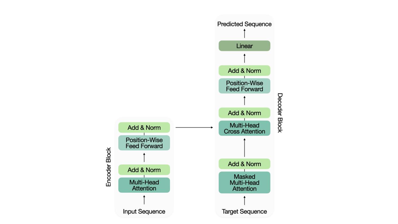
Figure 2. Model Architecture.

This project has adopted the transformer architecture proposed by Viswani et al. This model relies on the encoder and decoder blocks and the multi-headed attention mechanism to facilitate learning on sequential data.

3.4. Attention & Transformer Architecture

3.4.1. Self & Cross Attention. The attention mechanism is central to modern models like transformers, which rely on calculating attention scores to determine the importance of each part of the input data. This enables the model to intuitively focus on crucial parts of the data for prediction. The attention mechanism is based on three core components: keys (K), queries (Q), and values (V), which are extracted as vectors from the input data through a linear transformation. The attention score is calculated in (1):

\( Attention=softmax(\frac{Q\cdot {K^{T}}}{\sqrt[]{{d_{k}}}}+M)\cdot V \) (1)

In self-attention, the model calculates the relationships within the input sequence, enabling it to capture dependencies between different parts of the data. Cross-attention, used in encoder-decoder architectures, processes queries from the decoder and keys/values from the encoder, focusing the decoder on relevant input data to improve prediction accuracy.

The transformer’s encoder consists of multi-headed self-attention blocks, a dropout layer, layer normalization, and a position-wise feedforward network. Multi-headed attention allows for parallel computation of different patterns, while dropout prevents overfitting. Layer normalization stabilizes learning by standardizing the output data, and the position-wise feedforward network introduces the necessary non-linearity through ReLU activation.

The decoder mirrors the encoder but includes an additional masked multi-headed attention block, which restricts the model from looking ahead at future data during predictions. The decoder also features a cross-attention block, where queries from the decoder attend to keys and values from the encoder. This two-level attention mechanism allows the model to refine predictions based on both the input sequence and the target data.

Figure 3. Multi-Task Learning.

3.4.2. Multi-Task Encoding/Decoding. For a multi-task model, where the model tries to predict more than one output simultaneously, the encoding and decoding of the input sequences are handled differently. Each task, such as global temperature and greenhouse gas emissions, has an independent encoder, which allows the model to learn the interdependencies among each task individually. The outputs of each encoder are then concatenated to match the shape of the target prediction, which includes the data from both tasks. The decoder then performs self-attention on the outputs of both tasks, learning the relationship between the target sequences and the relationship within a prediction sequence. The cross-attention module is across both tasks, taking the concatenated outputs of both encoders, which allows the decoder to make predictions for both tasks simultaneously based on how the outputs of each task relate to others.

4. Experimental results

4.1. Datasets

In this study, I used two primary datasets for the global temperature prediction task: one focused on global temperature anomaly (NOAA Global Surface Temperature) and the second on global greenhouse gas emissions.

4.1.1. NOAA Global Surface Temperature (NOAAGlobalTemp). I chose the NOAA Global Surface Temperature dataset version 5.1, provided by the National Centers for Environmental Information for global temperature [13]. The data combines both land and sea surface temperatures, providing a holistic view of the global temperature, and also includes a variety of location ranges, including one that extends from 90S to 90 N. Although the dataset provides additional data, such as the total, high-frequency, and low-frequency error variances, I will focus mainly on the temperature anomaly provided in Kelvin for this project.

4.1.2. \( {CO_{2}} \) and Greenhouse Gas Emissions. The link between greenhouse gas emissions and global temperature cannot be stressed enough – especially \( {CO_{2}} \) . The second dataset pertains to global greenhouse gas emissions curated by Our World in Data [14]. This dataset collects greenhouse gas emissions from most contributing countries and also the global cumulative emissions of greenhouse gasses. Measured in tonnes of carbon dioxide equivalents, this dataset offers insights into the historical and current trends of emission data. For this project, I will focus on the global emission data, an aggregate of the constituent countries.

4.1.3. Preprocessing. Due to the large amounts of data, data processing was required to ensure an efficient training loop. For the NOAA Global Surface Temperature data, I isolated the anomaly of the temperature variable and the timestamp (year, month) into a data frame. This simplification was crucial for streamlining the data processing. Then, I was able to design a custom data manipulation tool in Python intended to segment the data according to specific temporal parameters. The tool was created with flexibility in mind, allowing for adjustable input and output years to accommodate different types of training. I opted for a configuration with a ten-year input sequence and a one-year output sequence to train my model. I wrote a custom Pytorch Dataset class for the time series data, designed to handle the loading of the time series data and the input and target tensors. Utilizing Pytorch’s built-in split functionality on my custom dataset, I segmented my data into train, validation, and test datasets.

Figure 4 visualizes the differences between non-overlapping and overlapping segmentation. From the figure, different input and target sequences could contain the same data, causing redundancy in the training, validation, and testing sets.

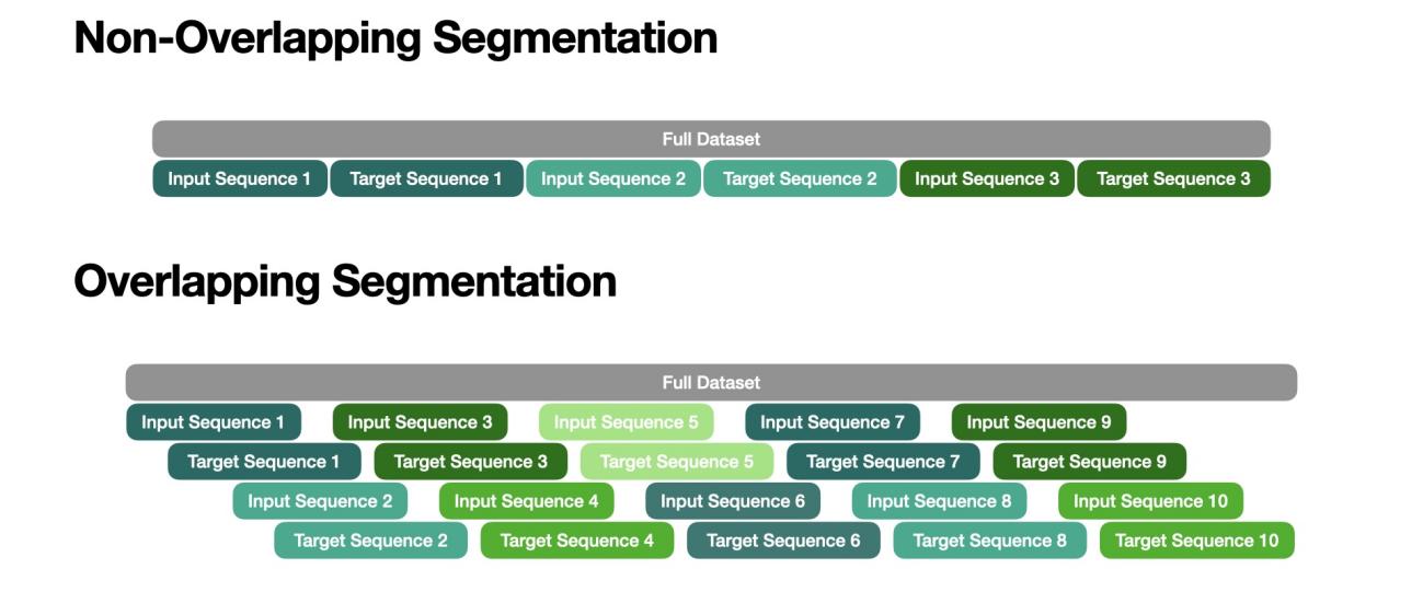
Figure 4. Non-Overlapping and Overlapping Segmentation.

For the multi-task learning with the NOAA Global Surface Temperature data and the CO \( {​_{2}} \) and Greenhouse Gas Emission data, I had to ensure they both followed an annual timeframe. The temperature data was initially available in a finer, monthly temporal resolution; I had to aggregate the global temperature anomaly data every twelve months and ensure it aligned with the greenhouse gas emission data. The greenhouse gas emission data presented a different challenge due to the data’s scale. A StandardScalar transformation from the ScikitLearn library was applied to the emissions data to address this. This scaling standardizes the data by introducing a mean of zero and scaling to a constant variance, ensuring that the magnitude of the emissions data is comparable to the temperature data during the multi-task learning process. This normalization is crucial to maintain the balance between the two inputs, ensuring that one input feature does not dominate the model due to its scale. In addition, because the temporal resolution was now annual, I updated the prediction to input ten years and output ten years.

In addition, to accommodate the multi-task learning process, it was necessary to ensure that both datasets had the exact dimensions and number of features. Since the temperature data included multiple location ranges and the greenhouse gas emission data did not, they had to be aligned. This was achieved through a padding process, where additional "dummy" features were added to the emissions dataset to match the global temperature data. This was essential for multi-task learning as it requires a consistent input shape across all tasks to learn to share and task-specific calculations that go into training.

4.2. Metrics

To effectively evaluate the model’s performance in predicting global temperature anomalies, \( {CO_{2}} \) , and greenhouse gas emissions, I have decided to use a comprehensive set of metrics that offer unique insight into different aspects of the model’s accuracy and reliability.

4.2.1. Loss Function (MSE). The primary metric used during the model’s training and optimization process is the Mean Squared Error (MSE), a standard loss function for regression tasks. MSE calculates the average squared difference between the model predictions and the ground truth, as defined in (2).

\( MSE=\frac{1}{n}\sum _{i=1}^{n}{({Y_{i}}-{\hat{Y}_{i}})^{2}} \) (2)

In (2), \( {Y_{i}} \) represents the actual values, \( {\hat{Y}_{i}} \) denotes the predicted values that are the model output, and \( n \) is the number of observations, i.e., the temporal frames. The MSE calculation penalizes significant errors through backpropagation, making it sensitive to sudden outliers and aiming for an accurate prediction.

4.2.2. Evaluation Metrics. In addition to the Mean Squared Error loss function, I have chosen a few more metrics to quantify the model’s generalization performance. These metrics are not used in training but only for testing and evaluation. They include the root mean squared error (RMSE), the mean absolute error (MAE), and the coefficient of determination ( \( R2 \) score).

Root Mean Squared Error (RMSE)

The RMSE is the square root of the MSE and measures the error’s average magnitude, as defined in (3). In contrast with the MSE, the RMSE is presented in the same units as the target variable and offers a more interpretable measure of the model’s performance for an external viewer.

\( RMSE=\sqrt[]{MSE} \) (3)

Mean Absolute Error (MAE)

MAE measures the average magnitude of the errors in a set of predictions without considering the direction (if the forecast is greater or smaller than the ground truth). It is calculated as the average of the absolute differences between the predicted and observed values – a straightforward measure of the prediction accuracy. The MAE is less sensitive to outliers compared to the MSE.

\( MAE=\frac{1}{n}\sum _{i=1}^{n}|{Y_{i}}-{\hat{Y}_{i}}| \) (4)

Coefficient of Determination ( \( {R^{2}} \) Score)

The \( {R^{2}} \) score measures how well the model predicts the outcome and how the prediction fits the observed data. The calculation uses the sum of squares of residuals, the sum of the squared differences between the predictions and the ground truth, and the sum of squares, the sum of the squared differences between the ground truth and the mean of that sequence. \( {R^{2}} \) values range from 0 to 1, where higher values indicate higher model performance.

\( {R^{2}}=1-\frac{\sum _{i=1}^{n}{({Y_{i}}-{\hat{Y}_{i}})^{2}}}{\sum _{i=1}^{n}{({Y_{i}}-\overline{Y})^{2}}} \) (5)

In (5), \( \overline{Y} \) is the mean of the ground truth data. I can comprehensively assess the model’s accuracy and reliability by employing these metrics: MSE, RMSE, MAE, and an \( R2 \) score.

4.3. The results

This section will focus on visualizing our prediction results and comparing them. We trained the models with each configuration for 100 epochs.

4.3.1. Visualization of Prediction Results. Figure 5 highlights the ground truth data for reference, which are included to compare different prediction methodologies, single-shot and autoregressive predictions comprehensively. From the figure, we can see that the autoregressive model predicts the output sequence more accurately than the single-shot model.

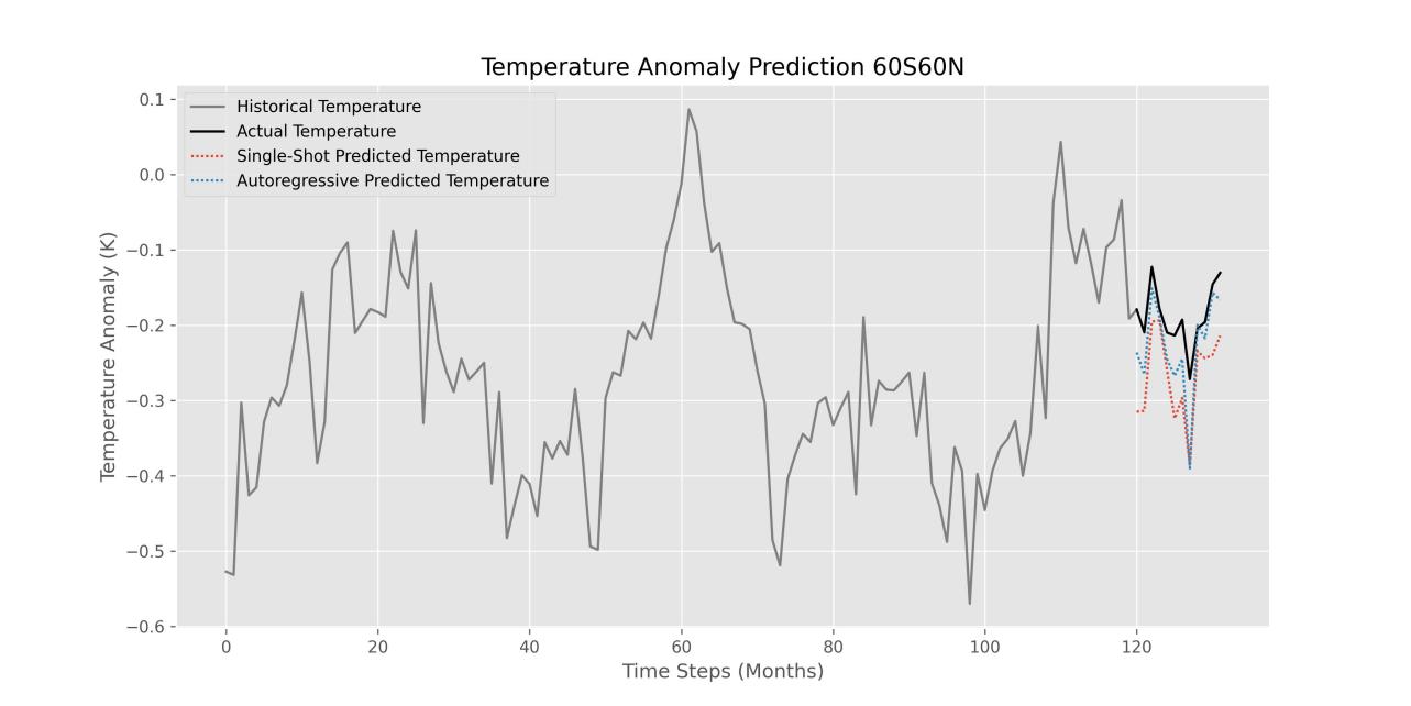
Figure 5. Prediction results for the Single-Shot & Autoregressive Models across different locations.

Figure 6 below visualize the prediction of the multi-task model. The input sequence is ten years, and the output sequence is also ten years. In the multi-task learning framework, it’s evident that the autoregressive model slightly outperforms the single-shot model in this location range.

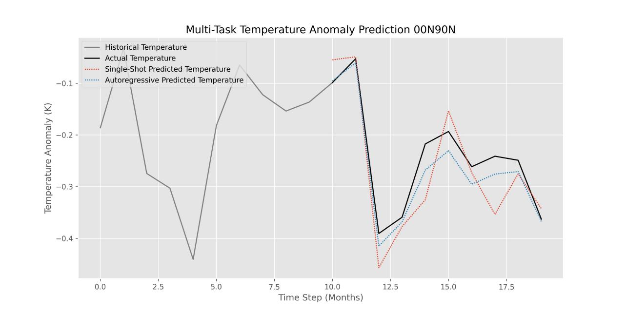
Figure 6. Prediction results for the Multi-Task Model.

4.3.2. Quantitative Results. In this subsection, I will focus on the quantitative results of my models, compare them to each other, and introduce the baseline model, the Informer, proposed by Zhou et al. [12].

4.3.2.1. Baseline Model (Informer)

The Informer model is a highly efficient, transformer-based architecture for Long Sequence Time-Series Forecasting. Its target is efficiency and speed without compromising prediction accuracy or reliability. It uses a ProbSpare Self-Attention Mechanism to save time compared to traditional Transformer models. This lowers the time complexity of the calculation, making this model more scalable for processing more significant inputs. Not only that, but this model uses a generative style decoder that predicts time series sequences in a single forward operation instead of an autoregressive approach.

4.3.2.2. Model Performance vs. Baseline

For this comparison, I will focus on the Informer and our single-shot and autoregressive methods, which have been trained with only temperature data (single-task) without any overlap in data. Our models share three metrics: MSE, RMSE, and MAE.

Table 1. Comparison of Custom Models to Informers

Figure 7 below shows a graphical comparison of these values.

Figure 7. Comparison of Informer Model Performances.

4.3.2.3. Single-Shot vs. Autoregressive: Our Model

The comparison between single-shot and autoregressive forecasting is pivotal to understanding how each approach processes. It predicts based on the temperature data under a single-task learning setting with and without data overlap. Without the restriction of a foreign model, we can use all of our additional metrics. Examining the MSE, RMSE, MAE, and \( {R^{2}} \) score for each model, we gain insights into the strengths and limitations of each method.

Table 2. Comparison of Single-Shot to Autoregressive Models

4.3.2.4. Impact of Data Overlapping

Another crucial comparison concerns the impact of data overlapping on model performance. Overlapping data segments can introduce redundancy and increase the model’s training time. On the other hand, overlapping data could also produce more data for training, making the model more robust as it learns more. This analysis highlights the trade-offs involved in data preparation, providing insight on how to optimize the training process. Figure 8 below compares the four single-task models, comparing the models trained on overlapping data to those not.

Figure 8. Comprehensive Model Comparison.

4.3.2.5. Single-task vs. Multi-task: Our Model

One of our main focuses is the difference in predictive power in single-task versus multi-task learning. Does a model optimized for a specific forecasting task outperform a model trained to perform multiple forecasting tasks simultaneously? The multi-task approach promotes the learning of more generalized features. It encourages the model to explore, identify, and exploit dependencies between the tasks, potentially leading to improved performance on individual tasks. The visualization would be impractical since the single-task and multi-task models are trained with different temporal resolutions. However, by examining key metrics such as MSE, RMSE, MAE, and the \( {R^{2}} \) score across both learning frameworks, we can assess the impact of multi-task learning on the model’s ability to predict temperature data since that is the common link. There is no data overlap, and the models are trained for 100 epochs each. Table 3 and figure 9 displays these metrics graphically.

Table 3. Comparison of Single-Shot to Autoregressive Models

Figure 9. Single and Multi-task Model Comparison.

4.3.2.6. Impact of Model Size

Exploring the impact of the model size, more precisely the number of encoder and decoder layers is an integral aspect of our analysis. One of the significant hyperparameters is that as models become more complex with increasing layers, their capacity to learn patterns changes depending on the data. Usually, as a model becomes more complex, their ability to identify interdependencies generally improves. An overly complex model can easily overfit a dataset, learning the noise and often trivial and irrelevant information. This can lead to decreased performance of models with a higher complexity. In this study, I have decided to focus on the complexity of the single-task model. We can observe their performance across our additional metrics by systematically adjusting the number of encoder and decoder layers in our models. This comparison provides insight into the trade-offs between a higher model complexity and forecasting accuracy.

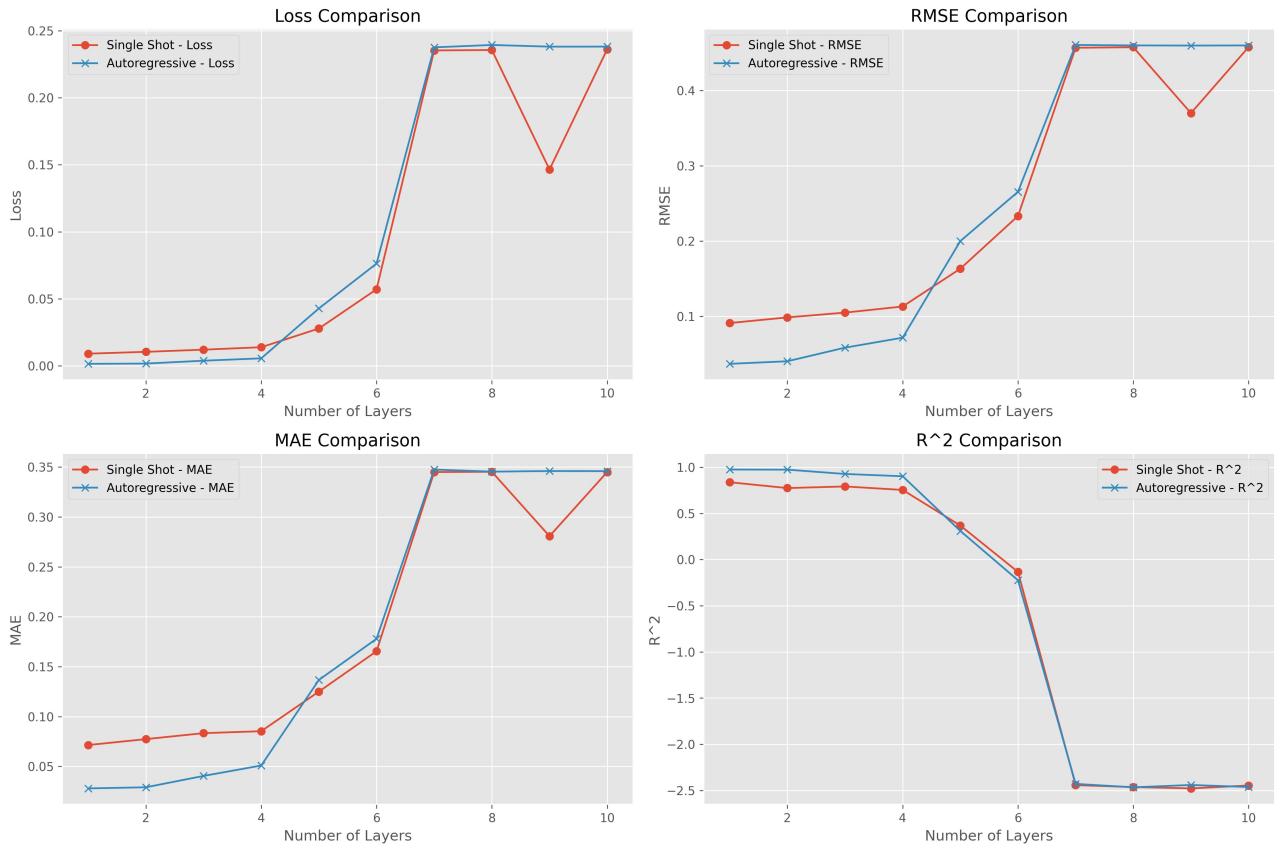
Figure 10. Model Size Comparison.

5. Discussion

This section discusses the experimental results, providing insight and interpretations beyond the data presented in the results section.

5.1. Single-Shot vs. Autoregressive

The distinction between single-shot and autoregressive models makes them extraordinarily different, producing drastically different results in time series forecasting. Single-shot models, with the ability to predict an entire sequence in one operation, are more computationally efficient and avoid accumulative errors. However, there is a slight cost of prediction performance, as most of the metrics show that autoregressive predictions are more favorable in almost every condition. By leveraging their previous outputs as inputs for subsequent predictions, autoregressive models can adapt to the changing nature of time series. Also, autoregressive models can be applied to an altered temporal resolution without having to be retrained. Their performance comes at a risk of error accumulation over time but can be fixed through longer training times and more data.

The results show that autoregressive processes usually outperform the single-shot calculations. On a shorter temporal resolution, 12 months and ten years, the error accumulation is almost nonexistent and is dragged down by the loss function through backpropagation. The precise and meticulous nature of the autoregressive models allows it to outperform the single-shot models in terms of time series forecasting.

5.2. Overlapping

Data overlapping (as suggested by my experimental results) plays a dramatic factor in time series forecasting. On the one hand, overlapped data segments can provide models with more context and more data to learn from, enhancing their ability to capture the patterns and dependencies present in the data.

However, excessive overlap can lead to redundancy and overfitting of the model. This means that data in the training set could also be in the validation and testing sets, making validation and testing almost meaningless, as the model has already seen the data. Finding the right balance between providing extra contextual information and avoiding redundancy is crucial in dataset preparation.

The experimental results suggest this exact conclusion. The models trained on overlapping data significantly outperformed those trained on non-overlapping data. This is mainly because the model has already seen most of the testing and validation data, giving it a better chance at evaluation.

5.3. Single-Task vs. Multi-Task

Discussing how single-task and multi-task models compare is essential to this project. A single-task model represents specialization on one specific task, which tends to push it to perform well at a single operation. They excel in capturing the patterns and intricacies of the task, but they can overlook the broader context in which the task exists. On the other hand, multi-task learning gives the model a broader context for it to learn. It uses shared representations across related tasks (temperature and greenhouse gas emissions) to enhance the model performance. It relies on the additional interdependencies between the two data mediums unavailable in a single-task environment. However, data normalization is required to ensure the model maintains a balanced focus across tasks, preventing specific tasks from dominating and ensuring stable learning.

The results show that multi-task learning outperforms single-task learning in both single-shot and autoregressive processes. This highlights the interconnectedness of these environmental variables, such as temperature anomalies and greenhouse gas emissions, making multi-task learning more accurate and reliable. However, it should be remembered that the temporal resolutions and data input dimensions are different. The single-task model predicts one year or twelve months of data, with an input of ten years or 120 months; the multi-task model predicts ten years of data, with an input of ten years of data.

5.4. Model Size

The number of encoder and decoder layers present in the transformer-based model architecture is crucial to ensure maximum performance. While larger models with higher complexity have the potential to learn more nuanced patterns in the data, they also face the risk of overfitting and increasing computational demands. Without regard to computational pull from the model, this project will focus on finding the highest-performing model size.

From our results, it is evident that a simple model is best for our situation. Escalating the number of layers of the model and introducing complexity seems to push the model to overfit the training data and perform poorly on the testing and validation data. Our tasks seem simple enough to be handled by a transformer architecture with just one encoder layer and one decoder layer.

It’s evident that all of these factors—the choice between single-shot and autoregressive models, overlapping data, single- and multi-task learning, and model size—play a pivotal role in shaping the overall performance and applicability of time series forecasting models. These dimensions would have to be considered holistically to fit any situation.

6. Conclusion

In this project, I thoroughly investigated the prediction accuracy and reliability of the transformer architecture in climate time series forecasting. Through meticulous experimentation, it is clear that an autoregressive model, trained through a multi-task learning framework, significantly improved the prediction accuracy. The multi-task learning process has highlighted the value that interconnected environmental factors can bring during training, helping the model capture the correlations and causal patterns within the data. The comparison with the baseline Informer model demonstrated the customized transformer’s efficiency capability regarding complex environmental factors. This study emphasized the profound effects that machine learning can have on environmental science. The ability to accurately and reliably predict global temperatures is crucial for creating strategies to adapt and mitigate climate change.

For future work, there are many available facets. I plan to work on distilling my complex transformer model into a smaller model (potentially be deployed on portable devices) without losing prediction accuracy. In addition, I can find additional environmental variables to train the model and see if more tasks will increase model prediction accuracy. I can also dig deeper into the overlapping data aspect of the project and experiment with different degrees of overlapping data to see if that will affect the prediction accuracy. It would also be ideal to visualize the results geographically since geographic specificity was introduced into the model.

References

[1]. NOAA National Centers For Environmental Information. 2023 was the warmest year in the modern temperature record. https://www.climate.gov/news-features/featured-images/2023-was-warmest-year-modern-temperature-record, 2024.
[2]. Rebecca Lindsey and Luann Dahlman. Climate change: Global temperature. https://www.climate.gov/news-features/understanding-climate/ climate-change-global-temperature, 2024.
[3]. Junze Zhang, Kerry K Zhang, Mary Zhang, Jonathan H Jiang, Philip E Rosen, and Kristen A Fahy. Avoiding the “great filter”: An assessment of climate change solutions and combinations for effective implementation. Frontiers in Climate, 4:1042018, 2022.
[4]. George EP Box, Gwilym M Jenkins, Gregory C Reinsel, and Greta M Ljung. Time series analysis: forecasting and control. John Wiley & Sons, 2015.
[5]. Liming Ye, Guixia Yang, Eric Van Ranst, and Huajun Tang. Time-series modeling and prediction of global monthly absolute temperature for environmental decision making. Advances in Atmospheric Sciences, 30:382–396, 2013.
[6]. Robert B Cleveland, William S Cleveland, Jean E McRae, Irma Terpenning, et al. Stl: A seasonal-trend decomposition. J. Off. Stat, 6(1):3–73, 1990.
[7]. Sepp Hochreiter and J¨urgen Schmidhuber. Long short-term memory. Neural computation, 9(8):1735–1780, 1997.
[8]. Kieran MR Hunt, Gwyneth R Matthews, Florian Pappenberger, and Christel Prudhomme. Using a long short-term memory (lstm) neural network to boost river streamflow forecasts over the western united states. Hydrology and Earth System Sciences, 26(21):5449–5472, 2022.
[9]. BASEL Y El-Habil and SAMY S Abu-Naser. Global climate prediction using deep learning. Journal of Theoretical and Applied Information Technology, 100(24):4824–4838, 2022.
[10]. Ashish Vaswani, Noam Shazeer, Niki Parmar, Jakob Uszkoreit, Llion Jones, Aidan N Gomez, L–ukasz Kaiser, and Illia Polosukhin. Attention is all you need. Advances in neural information processing systems, 30, 2017.
[11]. Emy Alerskans, Joachim Nyborg, Morten Birk, and Eigil Kaas. A transformer neural network for predicting near-surface temperature. Meteorological Applications, 29(5):e2098, 2022.
[12]. Haoyi Zhou, Shanghang Zhang, Jieqi Peng, Shuai Zhang, Jianxin Li, Hui Xiong, and Wancai Zhang. Informer: Beyond efficient transformer for long sequence time- series forecasting. In Proceedings of the AAAI conference on artificial intelligence, volume 35, pages 11106–11115, 2021.
[13]. R. S. Vose, B. Huang, X. Yin, D. Arndt, D. R. Easterling, J. H. Lawrimore, M. J. Menne, A. Sanchez-Lugo, and H.-M. Zhang. NOAA Global Surface Temperature Dataset (NOAAGlobalTemp), Version 5.1 [aravg.mon.land ocean]. NOAA National Centers for Environmental Information, 2023.
[14]. Hannah Ritchie, Pablo Rosado, and Max Roser. Co and greenhouse gas emissions. Our World in Data, 2023. https://ourworldindata.org/co2-and-greenhouse-gas- emissions.
Cite this article
Han,Y. (2024). EcoCast: Multi-Task Global Temperature Forecasting via Autoregressive Transformers. Applied and Computational Engineering,114,162-177.
Data availability
The datasets used and/or analyzed during the current study will be available from the authors upon reasonable request.
Disclaimer/Publisher's Note
The statements, opinions and data contained in all publications are solely those of the individual author(s) and contributor(s) and not of EWA Publishing and/or the editor(s). EWA Publishing and/or the editor(s) disclaim responsibility for any injury to people or property resulting from any ideas, methods, instructions or products referred to in the content.
About volume
Volume title: Proceedings of the 2nd International Conference on Machine Learning and Automation
© 2024 by the author(s). Licensee EWA Publishing, Oxford, UK. This article is an open access article distributed under the terms and
conditions of the Creative Commons Attribution (CC BY) license. Authors who
publish this series agree to the following terms:
1. Authors retain copyright and grant the series right of first publication with the work simultaneously licensed under a Creative Commons
Attribution License that allows others to share the work with an acknowledgment of the work's authorship and initial publication in this
series.
2. Authors are able to enter into separate, additional contractual arrangements for the non-exclusive distribution of the series's published
version of the work (e.g., post it to an institutional repository or publish it in a book), with an acknowledgment of its initial
publication in this series.
3. Authors are permitted and encouraged to post their work online (e.g., in institutional repositories or on their website) prior to and
during the submission process, as it can lead to productive exchanges, as well as earlier and greater citation of published work (See
Open access policy for details).