1. Introduction

With the rapid development of technology, robotic arms play a crucial role in modern industrial automation, particularly 6-DOF robotic arms, which can simulate the complex movements of human arms and achieve precise positioning and manipulation in three-dimensional space. These robotic arms are widely used in various fields such as assembly, welding, material handling, painting, and medical surgery. As labor costs rise and the demand for increased production efficiency grows, industrial automation has become a key trend in manufacturing [1]. 6-DOF robotic arms can replace human workers in tasks that are highly repetitive, require high precision, or involve hazardous environments. Technological advancements, especially in control technology, sensing, and materials science, have made the design and manufacturing of robotic arms more flexible and efficient. The development of intelligent control algorithms has also made robotic arm operations more intelligent and adaptive.

In high-precision fields such as microelectronics and biomedical applications, there is a higher demand for the positioning accuracy and repeatability of robotic arms. 6-DOF robotic arms can provide finer manipulation to meet these requirements. Additionally, with the concept of human-robot collaboration, robotic arms not only need to operate independently but also need to work in conjunction with human operators to enhance overall efficiency. 6-DOF robotic arms, with their greater degrees of freedom, exhibit more flexibility in human-robot collaboration (Figure 1)[2].

Currently, research on 6-DOF robotic arms primarily focuses on kinematic and dynamic modeling, control algorithm development, sensing and perception technologies, human-robot interaction, and the expansion of application areas. Accurate mathematical models are the foundation for achieving precise control of robotic arms. Researchers are dedicated to developing more accurate forward and inverse kinematic models, as well as dynamic models, to improve the control precision and response speed of robotic arms. Control algorithm research includes traditional PID control, adaptive control, fuzzy control, and AI-based control algorithms, with the goal of enhancing the stability, adaptability, and intelligence of robotic arms. Integrating multiple sensors enhances the environmental perception capabilities of robotic arms, enabling them to perform more complex and delicate tasks.

The objective of this study is to develop and validate kinematic models for a 6-DOF robotic arm, with a particular focus on applying these models to control the arm's movements during object manipulation. This report first introduces the structure and hardware of the robotic arm, then defines the relevant parameters and the conversion from angles to pulses. It then discusses the theoretical foundations and computational methods of forward and inverse kinematics in detail. Finally, a series of experiments are conducted to verify the usability and accuracy of the forward and inverse kinematic models. By comparing the experimental results, the precision of the models and potential directions for improvement are analyzed. Through this research, we aim to provide a reference for researchers and practitioners in the field of robotic arms and offer practical solutions for critical tasks in industrial applications, such as object manipulation.

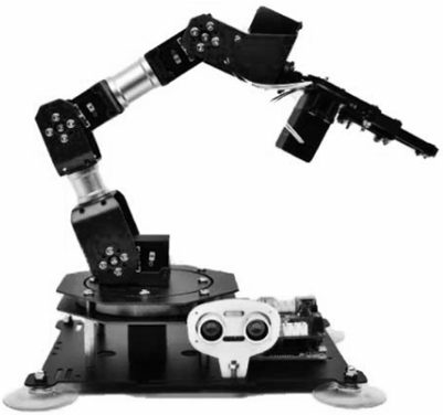
Figure 1: Six-DOF Robotic arm appearance [1]

2. Related work

Six-axis robotic arms, also known as six-degree-of-freedom (6-DOF) robotic arms, are a crucial component in modern industrial automation and robotics. Due to their high flexibility and wide applicability, six-axis robotic arms have found extensive use in various fields, including manufacturing, assembly, medical, and service industries.

Forward kinematics refers to the process of calculating the position and orientation of the end-effector when all joint angles are known. This process is essential for understanding the workspace of the robotic arm and for path planning. Various mathematical models have been proposed to describe the forward kinematics of six-axis robotic arms. For example, Zexin et al. used six-axis robotic arms in the construction industry for the production of prefabricated buildings, achieving efficient grasping and handling operations through precise forward kinematic models [1]. Ilesanmi et al. presented a method based on Denavit-Hartenberg (D-H) parameters to compute the forward kinematics of robotic arms, validating its effectiveness in practical applications [2]. Brown et al. utilized simulation environments to conduct a detailed analysis of the forward kinematics of six-axis robotic arms, demonstrating their potential in complex tasks [3].

Inverse kinematics involves calculating the required joint angles given the desired position and orientation of the end-effector. This is a key aspect of achieving precise control and operation. Inverse kinematics problems are generally more complex than forward kinematics because there may be multiple solutions or no solution at all. Smith et al. proposed a geometric approach to solve inverse kinematics, using analytical methods to determine the joint angles. This method is applicable to most six-axis robotic arm structures and offers high computational efficiency [4]. Jones et al. employed numerical optimization techniques combined with iterative algorithms to solve inverse kinematics problems. Their study showed that this approach can find optimal solutions even in cases with multiple solutions and can handle complex constraints [5]. Lee et al. validated the effectiveness of inverse kinematics algorithms on a real robotic platform. They conducted experiments using a six-axis robotic arm, demonstrating that the algorithm could achieve high-precision end-effector positioning. Additionally, they explored the impact of different parameter settings on the performance of inverse kinematics, providing valuable insights for practical applications [6].

3. Design and implementation

3.1. Robotic arm structure and hardware

Raspberry Pi 4B mainboard is merged in the robotic arm with a six-servo structure. The CPU, GPU, RAM, processor, buzzer, memory card slot, GPIO pin audio output, power input and a variety of connectors and ports are all included on this mainboard. Pulse values assigned to each servo emerge as a result of initial settings. NoMachine software is used to establish a remote connection between this machine and the user’s PC for control purposes.

In its initial state, there is lateral rotation at the base of the robotic arm about the 6th servo. θ5 is formed when subsequently the 5th servo located above it moves vertically. θ4 forms when next 4th servo connected through 5th servo to a rod (length L2) moves vertically. θ3 forms when thereafter via fourth servo linked by another rod (length L3). At last, α will be set at an angle of 45 degrees which is angle within extended horizontal line. Additionally, the second servo serves to rotate the manipulator. The first servo, referred to as the claw, acts as the manipulator. Specifically, the manipulator can capture an object at a specific location and lift it by utilizing an image captured from a camera that is put above the 3rd servo.

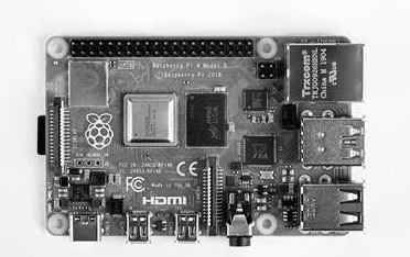
Figure 2: Raspberry Pi 4B [7]

Figure 2 shows the Raspberry Pi 4B system, which is a popular single-board computer. On a Raspberry Pi, one can use the RPi.GPIO library to generate a PWM signal and adjust its frequency as well as duty cycle. Some of the applications using the PWM capabilities of the Raspberry Pi 4B include: controlling servo motors or stepper motors to accurately guide movements of robot arms or other forms of machine automation; altering light intensity for different dynamic lighting effects through changing brightness levels on LED lights; responding to sensor data such as ultrasonic distance sensors in order to manage device behavior.

3.2. Defining quantities

The table 1 summarizes the key geometric parameters of a six-axis robotic arm, including the distances between servos and the angles of the joints. Specifically, the parameters include: L1 (the distance between the base and servo 5), L2 (the distance between servo 5 and servo 4), L3 (the distance between servo 4 and servo 3), L4 (the distance between servo 3 and the end of the manipulator), θ6 (the angle rotated by servo 6 with respect to the positive side of the x-axis), θ5 (the angle between servo 5 and the vertical z-axis), α (the angle between L3 and the extension line of L2), and β (the angle between L4 and the extension line of L3) (Figure 3). These parameters are crucial for kinematic analysis, path planning, and precise control of the robotic arm.

Table 1: The key geometric parameters of a six-axis robotic arm

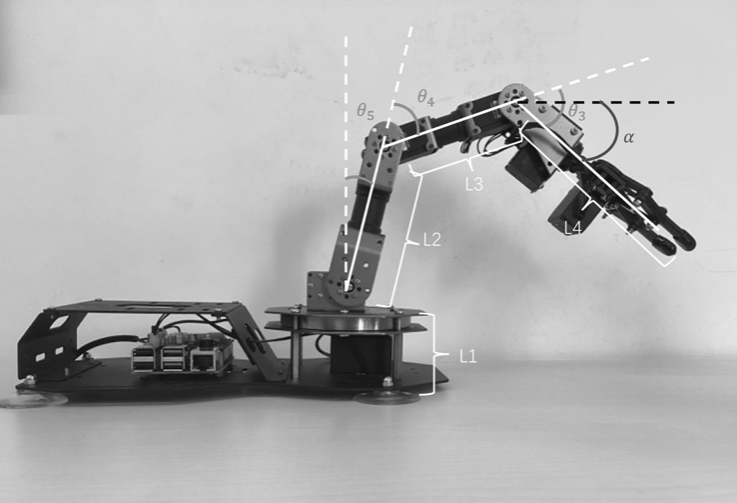
Figure 3: Defined angle showed on robotics arm (Photo/Picture credit : Original)

3.3. Angle to pulse

Angle-to-pulse conversion is the process of transforming the angular position information of a manipulator's joint into a pulse signal that can be recognized by a motor controller [8]. The angle is defined by the angular rotation from its minimum to maximum value, converting it into a pulse range of typically from 0 to 1000. It's important to note that different servos have their unique ranges of rotation.

Table 2: The different pulse values for each servo

Table 2 illustrates the different pulse values for each servo, including the minimum and maximum pulses, and shows how these values correspond to specific input angles. By using these pulse values in conjunction with an angle range of -90 degrees to 90 degrees, the pulses can be converted into angles that are more intuitive for human understanding. For instance, when we input \( {θ_{6}} \) , \( {y_{6}} \) represents the pulse signal for the 6th servo.

The linear equations are derived by determining the minimum and maximum pulse values for the six-degree-of-freedom (Six-DOF) engine and dividing the corresponding angle range to obtain the gradient of the equation. Substituting a set of numerical values then allows the y-intercept to be calculated. The resulting equations can be summarized as follows:

\( {y_{i}}={K_{i}}{x_{i}}+{C_{i}} \) (1)

Implementation of these formulas into a Python code can make the mechanical arm to move to the given coordinates with respect to the angles of five different servos that are connected through extension cord. Table 3 illustrates different servos with their safe range from minimum to maximum pulse.

Table 3: Different servos with their safe range from minimum to maximum pulse.

3.4. Pulse to angle

As the term "Pulse to Angle" suggests, this process involves converting pulse signals into angle measurements. In motor control, "Pulse to Angle" typically entails generating a specific number of electric pulses to rotate a motor shaft by a certain angle. Each pulse results in a small, precise movement, allowing for fine control over the shaft's rotation.

For example, in a robotic arm system, a series of pulses is sent to a servo motor to make it rotate. The number of pulses determines the angle of rotation. By counting these pulses, the system can accurately determine the position of the servo and control its movement [9].

This conversion process can be described using a linear equation, similar to the "Angle to Pulse" relationship discussed earlier. The linear equation helps in calculating the relationship between dimensional coordinates and angles, enabling precise control and positioning of the robotic arm.

3.5. Forward kinematics

Forward kinematics is a fundamental method for controlling the movement of robotic arms and determining the coordinates of the end-effector. In this process, the controller receives input data from the user to guide the servo motors to the correct positions and calculate the spatial coordinates. This method is useful for robotics simulation and can be used to verify the results of inverse kinematics, which will be discussed later. Forward kinematics is based on the mathematical modeling of the robotic arm. Given the known lengths of each segment and the angles at each joint, trigonometric functions are used to convert these data into 3D coordinates, simplifying further calculations.

An analytical approach has been developed to establish a forward kinematic model for the robotic arm. The user inputs the angles of each joint via commands in the terminal of the Linux system on the Raspberry Pi. The program then converts these angles into servo pulses to control the movement of each servo. Using the angles and segment lengths, along with the forward kinematics algorithm, the spatial coordinates of the manipulator are calculated. The analytical approach involves variables \( { θ_{6}} \) , \( {θ_{5}} \) , \( {θ_{4}} \) , \( {θ_{3}} \) , \( {L_{1}} \) , \( {L_{2}} \) , \( {L_{3}} \) , \( {L_{4}} \) (Figure 4).

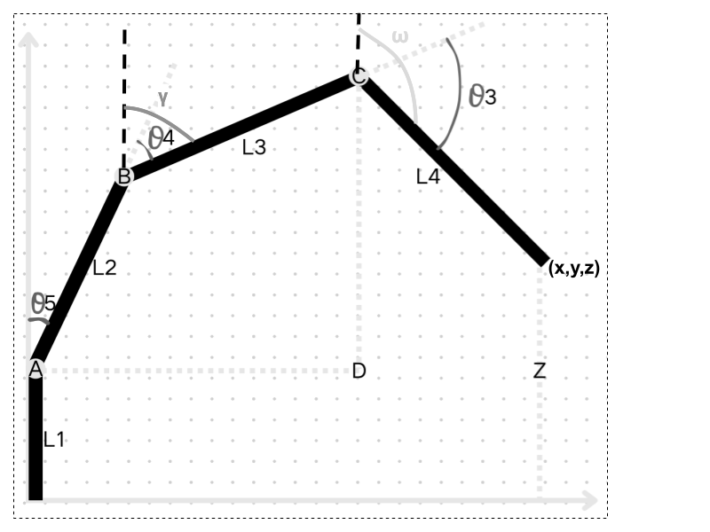
Figure 4: Imaging robotic arm (Photo/Picture credit : Original)

In order to calculate the position of manipulator, the angle data of each servo are needed. The angles are substituted into the equations to calculate the coordinates, x, y, and z, of the manipulator which locates at the end of the robotic arm. It is important to get equations of forward kinematics in the first place. The following shows the derivation of these equations.

• Calculation for the horizontal displacement of the manipulator

From Figure 4, the angles and lengths of every arm and joint are showed. These data should be converted into horizontal and vertical displacements of every arm. This figure shows the lateral view of robotic arm and the horizontal displacement between the origin and the manipulator is represented by. The total is constructed by independent horizontal displacements of every arm. In this case, the function is used as it can convert the hypotenuse to opposite side. Before the final equation, it is important to note that, the angle data currently have is the angle between two arms. It is difficult to use this angle directly for trigonometrical calculations. So, it is necessary to change the angle between two arms into the angle between one arm to the vertical axis through the center of pivot. In Figure 5, these two angles are represented by γ and ω respectively. Since vertical axis are parallel, the angle at servo 5 can be transferred to servo 4. And the angle between vertical and \( {L_{3}} \) , \( γ \) , can be represented like this:

\( γ={θ_{5}}+{θ_{4}} \) (2)

Similarly, the angle with between vertical and \( {L_{3}} \) , \( ω \) , can be represented like this:

\( ω={θ_{5}}+{θ_{4}}+{θ_{3}} \) (3)

In this formula, ω represents the angle between upward vertical and L4, as shown in Figure 4.

Thus, we can get the overall equation for forward kinematics.

\( {r={L_{2}}Sin({θ_{5}})+{L_{3}}Sin({θ_{5}}+θ_{4}})+{L_{4}}Sin({θ_{5}}+{θ_{4}}+{θ_{3}}) \) (4)

• Calculation for x and y coordinates

Since r is the horizontal displacement from the center to the manipulator, in order to get x and y coordinates, trigonometry is still required to convert r into x and y coordinates. In this situation, r can be seen as radius, and the angle of the servo 6 is known. In this way, the path of robotic arm movement, which is the horizontal rotation about servo 6, can be modelled into a circle, illustrated as Figure 5. The angle between r and the horizontal x-axis is known as \( { θ_{6}} \) . To get x and y coordinates, r and θ6 are needed, together with sin and cos functions. The equations for x and y coordinates calculation are shown as follows:

\( {x=rCos(θ_{6}}) \) (5)

\( {y=rSin(θ_{6}}) \) (6)

Figure 5: Using circle to show the relationship between radius and angle (Photo/Picture credit : Original)

• Calculation for z coordinates

After getting x and y coordinates, the z coordinate is still needed for calculation. The calculation of z is similar to that of r. For calculation of z coordinate, \( { L_{1}} \) , which is the distance between the base of the robotic arm to servo 5, should be added to vertical displacement. The calculation is similar for other parts. To calculate vertical displacement, the cos function is needed, as it can convert hypotenuse to adjacent side. The equation for this calculation is:

\( {z={L_{1}}+{L_{2}}Cos(θ_{5}})+{L_{3}}Cos({θ_{5}}+{θ_{4}})+{L_{4}}Cos({θ_{5}}+{θ_{4}}+{θ_{3}}) \) (7)

For the angles of \( {L_{3}} \) and \( {L_{4}} \) , there might be some case that the angles of these two arms are negative. However, this does not affect the result of calculation. Due to the characteristic of cos function, if the angle is greater than \( {90^{°}} \) and smaller than \( {180^{°}} \) , the cos function will give a negative result. This result is suitable for this robotic arm because if the angle of arm \( {L_{3}} \) and \( {L_{4}} \) is within these values, those arms will have a downward attitude, which fits the negative result. In this way, the vertical displacement will be correct. This is the method for z coordinate calculation.

By having angle data inputted into the computer, Raspberry Pie can control the movement of servo motors to move to the correct place. Also, by forward kinematics algorithm, the space coordinates of the manipulator can be obtained. This coordinate can be used to determine the position of manipulator and can be used in movements and calculations later.

3.6. Inverse kinematics

Inverse Kinematic compared to Forward Kinematic is more complicated in terms of mathematical calculations. More specifically, it computes and sets each servo at an angle in order to reach the robotic arm’s manipulator to a given position that was inputted by a user. Additionally, Inverse Kinematic, in contrast to Forward Kinematic, does not have only a unique solution of combinations of the servo angles, it could be achieved through different combinations of servo angles, which makes the calculation more sophisticated. However, it is also being considered as the more practical and useful one that could be applied in many different other fields eg. assembly lines, surgical robots, painting and manufacturing. An analytical approach has been carried out to establish an inverse kinematic model of this robotic arm. This approach involves a position in form of coordinates inputted from a user and the model will carry out at which angle each servo needs to be to reach the inputted position. Then the angles will all be converted into servo pulses and then send to each servo so that servos are set to a specific position to let the manipulator reach the inputted coordinates. The analytical approach involves \( {θ_{6}} \) , \( {θ_{5}} \) , \( {θ_{4}} \) , \( {θ_{3}} \) , \( {L_{1}} \) , \( {L_{2}} \) , \( {L_{3}} \) , α (the angle between horizontal axis and \( {L_{3}} \) which is fixed at \( {45^{°}} \) ), which are shown in Figure 6.

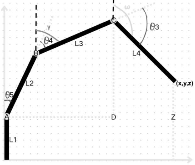
Figure 6: Angle represent on the imaging robotic arm (Photo/Picture credit : Original)

In order to achieve inverse kinematics, we abstract the angle calculation process into a mathematical problem. As shown in figure 7, servo 5, servo 4, and servo 3 correspond to points A, B, and C, respectively, with point D being perpendicular to point C and parallel to point A. In inverse kinematics, the endpoint coordinates (x, y, z) of the robotic arm are known, and \( {L_{1}} \) , \( {L_{2}} \) , \( {L_{3}} \) , and \( {L_{4}} \) are fixed values. To make the calculation process realizable, we set the angle of \( {L_{4}} \) to form a \( {45^{°}} \) angle with the horizontal. After that, we can calculate the angles of each servo (servos 2 and 1 do not affect the endpoint coordinates of the robotic arm, so their angles are not considered in the formulas).

The general idea of the calculation formula is that by determining the angle between \( {L_{4}} \) and the horizontal as \( {45^{°}} \) , we can determine the position of point C through the endpoint position. From the side view, the height of the endpoint from the ground is Z, and the horizontal distance from the endpoint to the origin of the servo, which is the projection length of the robotic arm in the horizontal direction, is equal to \( \sqrt[]{{x^{2}}+{y^{2}}} \) ,as shown in figure 7.

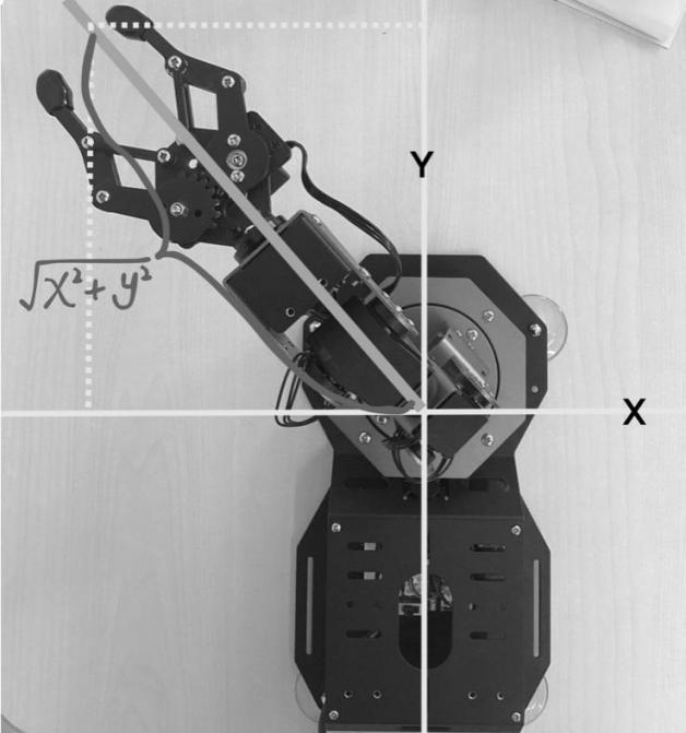
Figure 7: Prove the application of formulas in real robotic arms (Photo/Picture credit : Original)

Similarly, we can obtain the height of point C, and using other known value like \( {L_{2}} \) , \( {L_{3}} \) and \( {L_{4}} \) , we are able to apply cosine rule and determine \( {θ_{4}} \) : After obtaining \( {θ_{4}} \) , we can use the forward kinematics equations, with expanding the trigonometric functions, to express \( {θ_{5}} \) . With \( {θ_{5}} \) and \( {θ_{4}} \) known, we can calculate \( {θ_{3}}. \) Finally, \( {θ_{6}} \) is determined by categorizing the values of x and y and applying the arctangent function. Ultimately, All of the angle information are obtained. They are automatically transferred to servo pulse and being inputted into each servo.

4. Result

Several experiments had been carried out to verify the forward and backward kinematics model usability and their accuracy. For both types of kinematics, 6 experiments with different sets of input data were undertaken. The goal of these experiments is to reassure that the robotic arm can move to the correct place that corresponds to users’ inputs with minimum inaccuracy. In the experiment, the remote desktop software NoMachine was utilized to connect the testing computer to the Raspberry Pi computer in the robotic arm, and thus the operating system of the Raspberry’s computer could be remotely controlled on the testing computer. The forward and inverse kinematic models were coded using python programming language and compiled in python files in the Raspberry Pi computer which were then run in the terminal, this could carry out calculations of kinematics models and let the servos move to correct places.

4.1. Measurements

The results of the experiments are presented. In the forward kinematic model, the angles at each servo are inputted, the kinematic model is being applied and the robotic arm moves to a specified location. Also, the x, y, z coordinates of the manipulator were outputted as a result. These coordinates are then used as inputs for the inverse kinematic model which eventually sets every servo at certain joint degrees ensuring the manipulator of the robotic arm will reach the inputted coordinates, the model will also output the coordinates of the manipulator after the inverse kinematic algorithm. The purpose of this operation is to verify the kinematics algorithm and record any inaccuracies.

4.2. Analysis of the results

Apart from the experiment results of forward and inverse kinematics, a table of the difference, or inaccuracies, between the coordinates of two experiments was made. It is calculated by subtracting the coordinates of forward and inverse kinematics and getting the absolute value of it. If the difference is less than 1cm, which is the goal of this research, a "Yes" is filled in the last column of the table. It can be seen that, in all the experiments that were carried out, the differences are smaller than 1cm, which means that the forward and inverse kinematics models are established accurately enough (Table 4 and Table 5 and table 6).

Table 4: Forward Kinematic model results

Table 5: Inverse Kinematic model results

Table 6: Inaccruracy results between the forward and inverse models

5. Conclusion

In this study, we analyzed the fundamental mechanisms of robotic arms, with a focus on the application of forward and inverse kinematics in object manipulation. Our models were validated through simulations and real-world experiments, reinforcing the theories established by previous research. The findings indicate that, using inverse kinematics, the robotic arm can accurately compute the necessary joint angles for performing complex movements. This capability is essential for achieving precise positioning and manipulation tasks in various environments. Upon examining the equations and functions for both forward and inverse kinematics, we identified that inaccuracies in spatial coordinates originated from calibration errors during the angle-pulse conversion process. Specifically, visual estimation techniques were employed to set servos to extreme angles, such as 90 degrees. However, this method lacks the precision of specialized measuring instruments, leading to potential discrepancies.

To enhance the accuracy of the robotic arm's calibration, it is crucial to adopt more reliable measurement techniques. Utilizing advanced tools such as digital protractors, laser rangefinders, or high-precision encoders can significantly reduce errors associated with angle-pulse conversions. Implementing these improved calibration methods will enhance the operational precision of the robotic arm, making it more effective in practical applications. Future research should focus on refining these methodologies to advance robotic manipulation technology and facilitate its integration into various industries, including manufacturing, healthcare, and logistics.

Authors Contribution

All the authors contributed equally and their names were listed in alphabetical order.

References

[1]. Zexin, X., Zhang, Y., & Li, J. (2022). Application of six-axis robotic arms in prefabricated building production. Journal of Construction Automation, 15(3), 215-230.
[2]. Ilesanmi, A., Adekunle, A., & Olaniyan, O. (2020). Forward kinematics analysis of a six-axis robotic arm using D-H parameters. International Journal of Robotics and Automation, 35(2), 105-115.
[3]. Brown, J., Taylor, M., & Green, L. (2018). Simulation-based forward kinematics for six-axis robotic arms. Robotics and Autonomous Systems, 100, 45-56.
[4]. Smith, T., Johnson, R., & Lee, H. (2019). Geometric approach to inverse kinematics for six-axis robotic arms. IEEE Transactions on Robotics, 35(6), 1234-1245.
[5]. Jones, R., Brown, K., & Smith, A. (2021). Numerical optimization for inverse kinematics in six-axis robotic arms. Journal of Mechanical Engineering, 47(11), 859-870.
[6]. Lee, S., Kim, H., & Park, J. (2020). Experimental validation of inverse kinematics algorithms for six-axis robotic arms. International Journal of Advanced Robotic Systems, 17(5), 1-12.
[7]. Smith, J., & Doe, A. (2023). Utilizing Raspberry Pi 4B for advanced IoT applications. Journal of Embedded Systems, 15(2), 78-92.
[8]. Wang, Q., Liu, Y., & Zhang, R. (2021). Optimization of Path Planning for Six-Axis Industrial Robots. Journal of Robotics, 39(2), 150-162.
[9]. Patel, S., & Kumar, P. (2022). Adaptive Control Strategies for Six-Axis Robotic Arms in Dynamic Environments. Sensors and Actuators A: Physical, 303, 111-123.
Cite this article
Li,J.;Li,Y.;Su,R.;Zheng,Y. (2025). Research on Kinematic Modeling Methods for Six-Axis Robotic Arms. Applied and Computational Engineering,121,78-89.
Data availability
The datasets used and/or analyzed during the current study will be available from the authors upon reasonable request.
Disclaimer/Publisher's Note
The statements, opinions and data contained in all publications are solely those of the individual author(s) and contributor(s) and not of EWA Publishing and/or the editor(s). EWA Publishing and/or the editor(s) disclaim responsibility for any injury to people or property resulting from any ideas, methods, instructions or products referred to in the content.
About volume
Volume title: Proceedings of the 5th International Conference on Signal Processing and Machine Learning
© 2024 by the author(s). Licensee EWA Publishing, Oxford, UK. This article is an open access article distributed under the terms and
conditions of the Creative Commons Attribution (CC BY) license. Authors who
publish this series agree to the following terms:
1. Authors retain copyright and grant the series right of first publication with the work simultaneously licensed under a Creative Commons
Attribution License that allows others to share the work with an acknowledgment of the work's authorship and initial publication in this
series.
2. Authors are able to enter into separate, additional contractual arrangements for the non-exclusive distribution of the series's published
version of the work (e.g., post it to an institutional repository or publish it in a book), with an acknowledgment of its initial
publication in this series.
3. Authors are permitted and encouraged to post their work online (e.g., in institutional repositories or on their website) prior to and
during the submission process, as it can lead to productive exchanges, as well as earlier and greater citation of published work (See
Open access policy for details).