1. Background introduction

Diabetes is a metabolic condition characterized by excessive blood sugar and is one of the most dangerous chronic diseases. Diabetes can cause persistent damage to a wide variety of tissues, particularly the eyes, kidneys, heart, blood vessels, neurons, and nerve function. If a method that can effectively improve the accuracy of diabetes prediction and diagnosis is discovered, it will be able to detect and treat diabetes in its early stages using a variety of methods [1].

Because of the large number of indicators for diagnosis of diabetes, if it is to be analyzed from the group, the amount of data would be so large and the data may be missing. It is difficult to achieve satisfactory results by single machine learning model (LR, SVM). In recent years, the accuracy of most diabetes classification predictions has improved greatly. Karol Grudzinski used the KNN algorithm to make the accuracy of diabetes predictions reach 75.5% [2]. The accuracy rate obtained by the neural network is 75.4%, and the final rate of the classification prediction using the Bayesian method is 79.5%. The mixed neural network (Artificial Neural Network (ANN) and Fuzzy Neural Network (FNN) model) proposed by Allahverdi can reach to a much higher number, 84.24% [3]. Although the prediction accuracy obtained by using these models has improved step by step, in most experimental scenarios, the integrated learning method is better than the single machine learning model. In addition, although the Pima Diabetes dataset was used as a sample in most diabetes experiments, most of them did not detect and process data outliers during the data preprocessing phase, which greatly affected the final analysis results. Therefore, this paper proposes a hybrid prediction model based on K-Means outlier detection, synthetic minority oversampling technique (SMOTE) and Adaboost to analyze the diabetes data, so that the accuracy and AUC of the prediction model enhanced.

This paper will focus on the classification performance of various tree models, such as decision trees, random forests, random forests based on automatic parameter adjustment, and Adaboost based on hybrid models. Various types of tree model comparison goal are accuracy and AUC (Area Under Curve) baseline, these two indicators able to characterize the effect of the final classification of diabetes data. The structure of the full text is as follows. Next section will introduce the related work, the third chapter will carry out data preprocessing, modeling, test process description and test results analysis, the final conclusion will be stated in the fourth section.

2. Related work

2.1. K-Means outlier detection

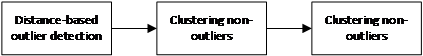
Clustering is a popular technique and is generally used to group data points in groups or clusters [4]. The K-Means algorithm based on the partitioning method has become the most widely used clustering algorithm because of its simple, fast and efficient processing of large-scale data. In this paper, the K-Means algorithm is used to detect outliers. K-Means clustering is an excellent outlier detection method. The core idea of the K-Means algorithm based on outlier detection is, firstly detect the outliers of the dataset by using the distance-based outlier detection method, and then randomly select K data points as clusters in the non-outliers. The initial seed uses the traditional K-Means algorithm to cluster non-outliers, and finally divides the outliers into corresponding clusters. The idea of the algorithm is shown in Figure 1.

2.2. SMOTE data balancing algorithm

SMOTE (Synthetic Minority Oversampling Technique), a new approach based on the random oversampling algorithm. The general classification data set has a large distribution difference between the number of most classes and a few classes. This phenomenon is called data imbalance [5]. Learning through unbalanced data sets is a problem that must be faced in supervised learning because the standard classification algorithm is designed to explain the balance class distribution. One such method is called oversampling, which creates a balanced class distribution by creating artificial data.

2.3. Decision Tree Model

The decision tree model is widely used in data classification for its ease of understanding, which was proposed by Quinlan [6]. The decision tree algorithm is a supervised learning algorithm that uses known answers and is used to build tree data. The most essential aspect influencing the quality of the results is the classification accuracy attained on the training dataset, as well as the size of the tree. Classification is the process of modeling different data categories while acquiring expected values for object categories or unknown properties during training on the dataset, and it is a vital duty of allocating objects to one of several predetermined categories. Decision tree algorithms that are currently accessible include ID3, C4.5, and CART. Each algorithm employs a distinct set of rules to select the optimum split for the goal of selecting the best constructing tree.

2.4. Boosting

Boosting is a landmark algorithm in the field of machine learning, which can improve the performance of any given learning algorithm. The "Probably Similar Correct" learning model proposed by Valiant in 1984 gave birth to the idea of Boosting. The concepts of strong learning algorithm and weak learning algorithm are defined in the PAC model [7]. If a learning algorithm learns a set of samples and the recognition rate is high, it's known as a strong learning algorithm. If the accuracy performance is only marginally higher than the random guess, which is 50%, it is a weak learning algorithm.

Boosting is a powerful technique for enhancing classification performance. The weak classifiers are recombined in a certain way to create a strong classifier with much enhanced classification performance. This approach successfully translates rough rules of thumb into highly accurate prediction rules. The strong classifier enhances the result of classifying data by voting and then pick the best number of votes on the weak classifier. The algorithm is a simple weak classification algorithm lifting process, which is continuously trained to improve the ability to classify data [8].

2.5. Adaboost

Freund and Schapire updated the Boosting algorithm in 1999, naming it the Adaboost algorithm, which does not demand prior knowledge about weak learning algorithms and has almost the same computing efficiency as Freund's Boosting algorithm proposed in 1991 [9, 10]. Adaboost is an acronym for Adaptive Boosting, which implements:

(1) The error rate of weak learning algorithms can be lowered using adaptive methods and mechanisms. The error rate can achieve the desired impact and goal after several iterations.

(2) The exact spatial distribution of the samples is not required. Adjusting the sample space distribution after each weak learning, updating the weights of all training samples, and reducing the weights of successfully categorized samples in the sample space can meet the objective. Misclassified sample weights are improved so that the next time when learned weakly, we will be more concerned with these misclassified samples. The algorithm can be easily applied to practical problems, so it has become the most popular Boosting algorithm.

The main principle of AdaBoost is to use the same training set to train multiple weak classifiers, and then combine these weak classifiers in a certain way to obtain a strong classifier.

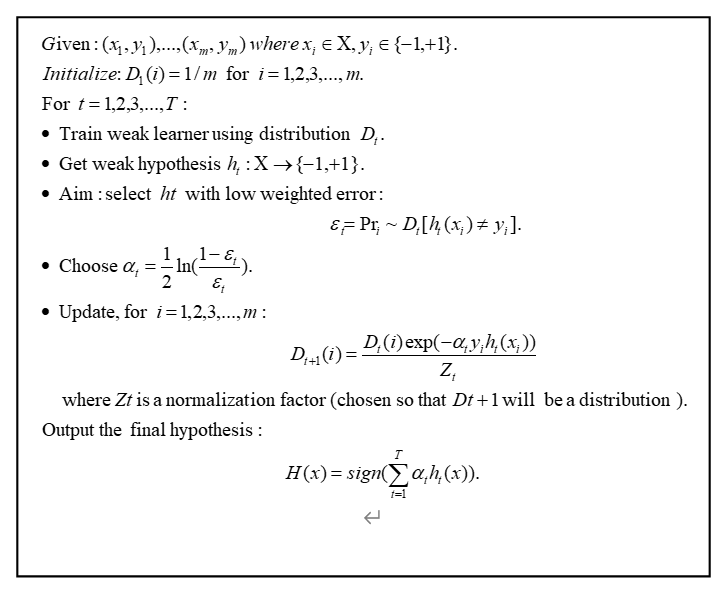
The process of AdaBoost is shown in Figure 2. This paper gives \( m \) as the training sample \( ({x_{1}},{y_{1}}),⋯({x_{m}},{y_{m}}) \) . In each round \( t=1,2,3,⋯,T \) , the distribution \( {D_{t}} \) calculates the m training samples as in Figure 2, and the given weak learning algorithm is used to find the classifier \( {h_{t}}:X→\lbrace -1,+1\rbrace \) , where the purpose of the weak learner is to find a classifier relative to \( {D_{t}} \) the weakly weighted \( {ε_{t}} \) error. The combined hypothesis \( H \) calculates a weighted classifier which shown in formular (1):

\( F(x)=\sum _{t=1}^{T}{α_{t}}{h_{t}}(x)\ \ \ (1) \)

This is said \( H \) to be a weighted majority vote that is calculated as a classifier, where each classifier is given a weight \( {α_{t}} \) .

3. Experimental analysis

This section uses a variety of machine learning algorithms to predict diabetes classification.

3.1. Dataset

The Pima Diabetes data used in this study was derived from the UCI public data set. The data consisted of 768 cases, divided into health data (500 cases) and disease data (268 cases), including 8 attribute values as shown in Table 1. To avoid overfitting and enhance the validity of the model, the diabetes data was separated into two sub-data sets in this experiment. One sub-data set was utilized for training, while the other was used as a test. The ratio of two sub-data sets is commonly 2:1. As a result, the training and test data sets contain 514 records and 254 records respectively. Finally, through the training data set, verify the performance of the test set on different classification algorithms to compare the advantages and disadvantages of each classification algorithm model.

Table 1. Property description.

3.2. Data pre-processing

To improve the precision of the final experimental results, data pre-processing is necessary. Since the collection process of the source data is uncontrollable, it leads to some outliers (e.g., blood pressure: 400), missing values, etc. In view of these situations, if the data is not pre-processed before data modeling, the resulting model will not perform well and affect the accuracy of the model. Therefore, data pre-processing is a very important stage in machine learning.

Data transformation and feature reconstruction: Data changes are regularization of the diabetes dataset, which can be trained and tested by normalizing the data to a uniform scale. In this dataset, this paper uses Z-score and MinMaxScaler for data regularization and convert all features into the given region. At the same time, the data features are reconstructed, and the regularized data features are taken as new features of the data set.

The equations provided in Equations (2) and (3) explain how to use regularization methods to transform data values.

\( MinMaxScaler(featur{e_{range}}=(0,1),copy=True)\ \ \ (2) \)

\( Z-Score(featur{e_{range}}=(0,1),copy=True)\ \ \ (3) \)

The equations provided in Equations (4), (5), and (6) explain the specific conversion steps.

\( {X_{std}}=\frac{X-{X_{.min}}}{{X_{.max}}-{X_{.min}}}\ \ \ (4) \)

\( {X_{scaled}}={X_{std}}*max-min+min\ \ \ (5) \)

\( Z-Score=\frac{(x-μ)}{σ}\ \ \ (6) \)

The final converted results are shown in Table 2. (Where Feature0 represents the pre-conversion feature and Feature represents the transformed feature).

Table 2. Transformed features name.

K-Means outlier detection: This experiment chooses 2 as the K value. That is because the "Outcome" variable contains two results, and the discrete point threshold is set to threshold=2. After iteration 500 times, the outlier point is finally detected and deleted. As shown in Table 3, this detection method greatly improves the final experimental accuracy.

Table 3. K_MEANS instance number before and after.

After 6 rounds of K-means outliers are removed, the data sets distributed in reasonable intervals are placed in the next training. Experimental results demonstrate that removing outliers can improve the accuracy of the final classification.

SMOTE data balance: The SMOTE algorithm can generate new samples by using the imputation formula (7).

\( {x_{new}}={x_{i}}+({\hat{x}_{i}}-{x_{i}})×δ\ \ \ (7) \)

When it is a random value between 0 and 1.

Finally, the proportion of positive and negative samples in the diabetes dataset (as shown in Table 4) is adjusted to 50%.

Table 4. Smote instance number before and after.

3.3. Modeling

In the above steps, this paper used K-Means for outlier detection, excluding the outliers from the data set, and then using the SMOTE algorithm to balance the data. After the data pre-processing step, this paper used 7 classifiers to train the data set. These classifiers include algorithms such as decision trees, SVM, Logistic Regression (LR), Random Forest (RF), Random Forest (RF) + GridSearch, Random Forest (RF) + Hyperopt, and Integrated Learning Algorithm (AdaBoost). In order to reduce the training test bias caused by data set partitioning, this paper used 50% cross-validation for training tests.

3.4. Experimental results

Tables 5 and 6 demonstrate the classification prediction results under two conditions. Table 5 represents the experimental results after data pre-processing using K-Means and SMOTE algorithms. Table 6 represents the experimental results using raw data and without any data pre-processing methods. The AUC, Accuracy, Precision, and Recall in table are used to measure the performance, and finally the A-C, Accuracy, Precision, and Recall can be applied to prove that the K-Means and SMOTE algorithms in the data pre-processing improve the final classification prediction.

The machine learning algorithm's classification rate or accuracy rate for true positives (TP-correct classification is true), false negatives (FN-error classification is false), true negative (TN-error classification is true), and false positives (FP- is correctly classified as false) are calculated as formular (8).

\( Accuracy=\frac{TP+FP}{TP+FP+TN+FN}\ \ \ (8) \)

The experimental evaluation index by combining K-Means and SMOTE technology is further improved than the evaluation index without using any data pre-processing method. As what can be seen from Table 5 and Table 6, for diabetes prediction, in addition to considering accuracy and AUC, Precision reflects the proportion of true positive samples in the positive example of classifier prediction, that is, can more accurately determine A sample of a suspected diseased group that is truly ill. Recall reflects the proportion of positive cases that the classifier correctly predicts to the total positive case. That is, it can measure the predictive ability of the classifier in the positive case of diabetes prediction. The larger the value, the stronger the positive predictive ability of the classifier. In Table 3, by comparison, the performance of the AdaBoost hybrid prediction model based on K-Means and SMOTE is the best. The values of the four metrics AUC, Accuracy, Precision, and Recall are 0.989, 0.950, 0.930, and 0.921. Compared with other classifier models, the model this paper proposed can not only accurately identify the diseased samples, but also make effective judgments on the true disease samples.

4. Conclusion

In this study, the research compares decision trees, support vector machines, logistic regression, random forests, random forests with GridSearch methods, random forests with the Hyperopt method, and AdaBoost classification results with K-Means and SMOTE methods, based on the Pima Diabetes dataset. The classification result shows that AdaBoost with K-Means and SMOTE methods can achieve the best results. It is because K-means can identify and help remove misinformation, and SMOTE can amplify the features of the data to a certain extent, thereby improving the training accuracy. It may be concluded and proved here that AdaBoost combined with K-Means and SMOTE approaches can significantly increase classification performance. At the same time, it solves the problem of inaccurate fitting caused by missing values and outliers. As the result, for classification issues, if the experimenter needs to select the tree model for data classification, it is recommended to use AdaBoost with K-Means and SMOTE methods for classification. From the perspective of optimizing this research, the number of dataset samples is still relatively small, requiring more experimental data to validate our proposed hybrid model. Because the existing clustering technology and the utilized data balancing algorithm still have certain defects. For instance, when use SMOTE to cluster, it may increase the degree of overlap between classes, and some samples that cannot provide useful information will be generated. Therefore, different data balancing algorithms and clustering algorithms will be used in the future to further improve the effectiveness of data pre-processing to improve the accuracy of the model and the metrics such as AUC.

References

[1]. Who.int. 2022. Diabetes. [online] Available at: <https://www.who.int/news room/factsheets/detail/diabetes> [Accessed 15 October 2022].Another reference.
[2]. Grudziński, K., 2008, June. Towards Heterogeneous Similarity Function Learning for the k-Nearest Neighbors Classification. In International Conference on Artificial Intelligence and Soft Computing (pp. 578-587). Springer, Berlin, Heidelberg.
[3]. Kahramanli, H. and Allahverdi, N., 2008. Design of a hybrid system for the diabetes and heart diseases. Expert systems with applications, 35(1-2), pp.82-89.
[4]. Madhulatha, T.S., 2012. An overview on clustering methods. arXiv preprint arXiv:1205.1117.
[5]. Chawla, N.V., Bowyer, K.W., Hall, L.O. and Kegelmeyer, W.P., 2002. SMOTE: synthetic minority over-sampling technique. Journal of artificial intelligence research, 16, pp.321-357.
[6]. Quinlan, J.R., 1996. Learning decision tree classifiers. ACM Computing Surveys (CSUR), 28(1), pp.71-72.
[7]. Valiant, L.G., 1984. A theory of the learnable. Communications of the ACM, 27(11), pp.1134-1142.
[8]. Freund, Y., Schapire, R. and Abe, N., 1999. A short introduction to boosting. Journal-Japanese Society For Artificial Intelligence, 14(771-780), p.1612.
[9]. Freund, Y. and Haussler, D., 1991. Unsupervised learning of distributions on binary vectors using two layer networks. Advances in neural information processing systems, 4.
[10]. Schapire, R.E., 2003. The boosting approach to machine learning: An overview. Nonlinear estimation and classification, pp.149-171.
Cite this article
Gao,H.;Zuo,D. (2023). Research on using AdaBoost with K-Means and SMOTE to predict the incidence of diabetes. Applied and Computational Engineering,6,67-73.
Data availability
The datasets used and/or analyzed during the current study will be available from the authors upon reasonable request.
Disclaimer/Publisher's Note
The statements, opinions and data contained in all publications are solely those of the individual author(s) and contributor(s) and not of EWA Publishing and/or the editor(s). EWA Publishing and/or the editor(s) disclaim responsibility for any injury to people or property resulting from any ideas, methods, instructions or products referred to in the content.
About volume
Volume title: Proceedings of the 3rd International Conference on Signal Processing and Machine Learning
© 2024 by the author(s). Licensee EWA Publishing, Oxford, UK. This article is an open access article distributed under the terms and
conditions of the Creative Commons Attribution (CC BY) license. Authors who
publish this series agree to the following terms:
1. Authors retain copyright and grant the series right of first publication with the work simultaneously licensed under a Creative Commons
Attribution License that allows others to share the work with an acknowledgment of the work's authorship and initial publication in this
series.
2. Authors are able to enter into separate, additional contractual arrangements for the non-exclusive distribution of the series's published
version of the work (e.g., post it to an institutional repository or publish it in a book), with an acknowledgment of its initial
publication in this series.
3. Authors are permitted and encouraged to post their work online (e.g., in institutional repositories or on their website) prior to and
during the submission process, as it can lead to productive exchanges, as well as earlier and greater citation of published work (See
Open access policy for details).