Pattern Recognition and Prediction

Yaoyu Chang; Zengjun Wei; Qizhen Cao

doi:10.54254/2755-2721/2024.20710

1. Introduction

Figure 1. Scatter Plot of x-y Coordinates for event 0

1.1. Background on pattern recognition and prediction

High-energy particle physics experiments are fundamental to exploring the building blocks of matter and the forces governing their interactions. These experiments typically involve colliding particles at extremely high energies, generating a multitude of secondary particles that travel through various detectors. Accurately reconstructing the trajectories of these particles is critical for understanding the physical processes at play. This reconstruction process hinges on three core tasks: vertex finding, track finding, and track fitting. Vertex finding is the first task that we have accomplished. The vertex represents the point of origin of the particle collision, typically located along the z-axis in the detector's coordinate system. By accurately determining the vertex is essential and important, because it serves as the reference point for our measurements. Following vertex finding, track finding involves identifying the paths taken by individual particles as they move through the detector. When it comes to track findings, we need to differentiate between multiple particle tracks, often in a dense and noisy environment with a lot of noise, where tracks may overlap or intersect with each other. The primary challenge for track finding is to correctly group the hits into coherent tracks, and then calculate and compute the momentum components of the particle in three dimensions x, y, z (px, py, pz). Track fitting, is a process where the raw estimates from the data are refined using mathematical models to describe the trajectory of the particle. In general, this entails fitting the hits associated with each track to a circle and gets better resolution for a particle. Improved track fitting does not solely help in having access to better-reconstructed tracks, but it also enhances this accessibility by being a smart filter of noise and controlled uncertainties that come with the measurements of pivotal physical parameters.

1.2. Research Objective

The primary objective of this research is to create and develop a robust and accurate algorithm or methodology for accurately performing vertex finding, track finding, and track fitting in the context of high-energy particle physics experiments. The key goals of this study are to account for the inherent challenges that come with noisy data, overlapping tracks, and precision momentum measurements. We combine classical geometric methods with different machine learning models like random forest regressor, MLP, and XGboost model in order to improve the transverse momentum ( $$ p_T $$ ) predictions to a large extent. Our approach is evaluated using a dataset containing simulated collision events, where the true vertex and track information are given and known. This allows us to compare our predicted values with the ground truth and help us to enhance our algorithm. Last but not least, the success and accomplishment of this research and study will contribute to more precise particle trajectory reconstructions, which are crucial and essential for analyzing and interpreting data in particle physics experiments and making it possible to lead to deeper insights into fundamental physics.

2. The Dataset

In the task of vertex finding, we have data that involves 10,000 events, and each event comprises 20 hits, where three coordinates x,y and z of the hits are given. Our algorithm aims to find the vertex, which is the origin point from where the particles are emanated. The true vertex is provided in the first line of the data file, allowing for verification of the accuracy and preciseness of our vertex-finding algorithm. A crucial first step is to ensure that the events in the data are properly read, then examine the distribution of the hits in 3D space. It is expected that the hits will be distributed across two concentric cylinders, with the vertex lying on a line at the center of these cylinders, aligned with our z-axis. This step serves as the foundation for our vertex-finding process, which is a critical component of the pattern recognition pipeline[1]. The second task focuses on track reconstruction. In this context, each line in the file corresponds to a single hit, with the format: event number, track number, track momentum components (px, py, pz), and hit coordinates (x, y, z). Each track consists of five hits, and for each event, there are 20 tracks. The goal is to correctly group the five hits corresponding to each track and determine the momentum vector $\mathbf{p} = (\lt code\gt px\lt /code\gt , \lt code\gt py\lt /code\gt , \lt code\gt pz\lt /code\gt )$ at the vertex. The transverse momentum, $$p_T$$ , which is proportional to the radius $$r$$ of the circular trajectory of the hits in the $$x$$ - $$y$$ plane, The transverse momentum $$ p_T $$ is calculated based on the radius $$ r $$ of the circular trajectory in the x-y plane. Specifically, the transverse momentum is computed as:

\begin{equation} p_T = \sqrt{p_x^2 + p_y^2} \end{equation}

where $$ p_x $$ and $$ p_y $$ are the momentum components of the particle. The transverse momentum $$ p_T $$ reflects the particle’s motion in the transverse direction after the collision.The transverse momentum $$ p_T $$ reflects the particle’s motion in the transverse direction after the collision [3]. By accurately identifying the five hits that belong to each track, one can determine both the radius and the direction of $\mathbf{p}$ at the vertex, located at $$(0,0,0)$$ in these events. The data file's format is conducive to direct import into a pandas DataFrame for further analysis and visualization of the hit coordinates, although other methods of data processing are also possible[2], [3]. The third task focuses on track fitting. In this stage, the data file provides the true transverse momentum $$ p_T $$ and the five points on each track. This allows for the implementation of track fitting techniques to accurately reconstruct the trajectory of the particles and determine the $$ p_T $$ from the given hits. By fitting the track, we refine the estimation of the particle's momentum vector at the vertex, ensuring that the computed $$ p_T $$ closely aligns with the true value. This task can be initiated independently of the track-finding process, enabling different team members to work on vertex finding, track finding, and track fitting simultaneously for a more efficient workflow [1].

3. Methods

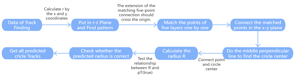
The method used in Vertex Finding is shown in Figure 2.

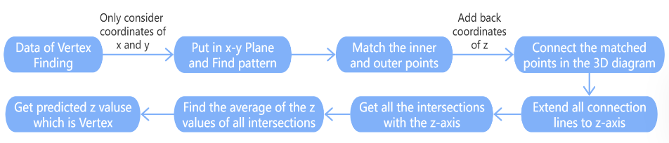
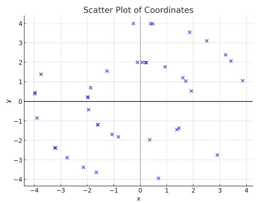
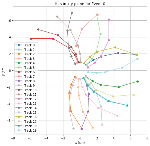
Figure 2. Flow chart of method in Vertex Finding

First take a set of events and observe the X-Y plane in the 2D graph. It was then discovered that the points formed two circles. (Figure 3 is an example of event 0 in Vertex Finding.)

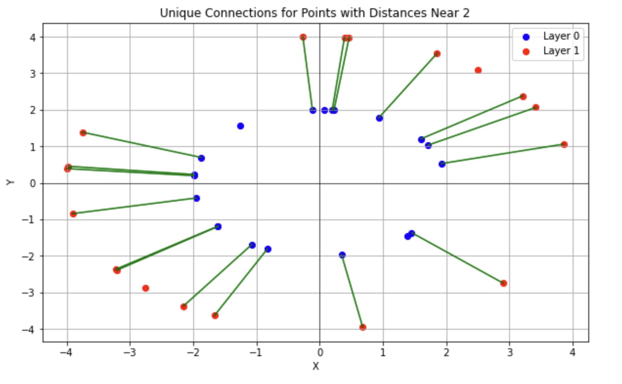
Figure 3. Scatter Plot of x-y Coordinates for event 0

In addition, we connect the inner points and the outer points one by one to eliminate interference points by checking whether the distance between the two points is near 2. (Figure 4 is an example of event 0 in Vertex Finding.)

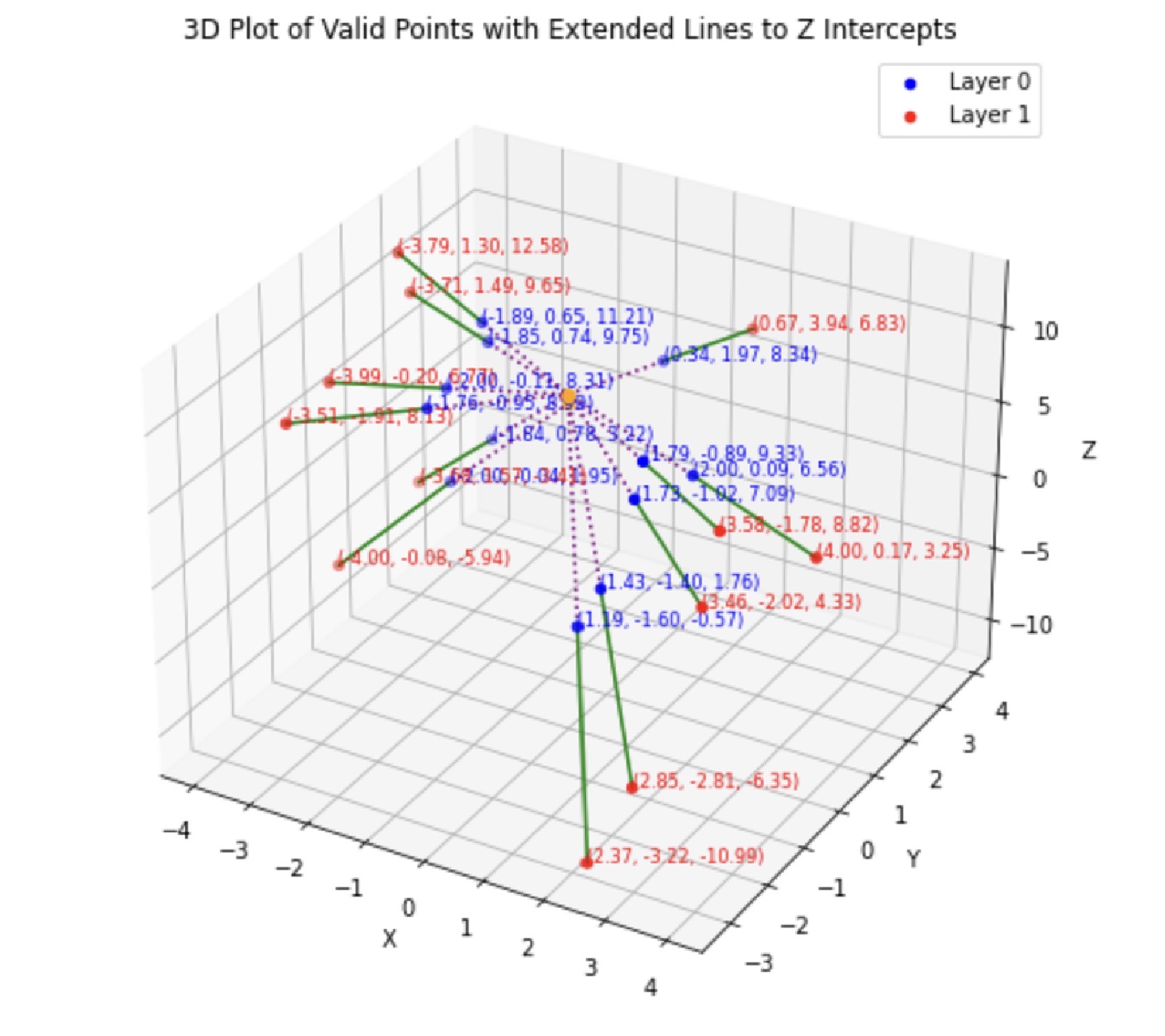
Figure 4. Unique Connections for points with Distances Near 2 for event 0

After the points on the two layers are corresponding, add the z-coordinates of the points and put them into the 3D map. Connect the corresponding points and extend the connection to see the point that intersects with the z-axis. (Figure 5 is an example of event 3 in Vertex Finding.)

Figure 5. 3D Plot of Valid Points in event 3 with Extended lines to Z intercepts

Finally, the mean of the intersection points of these lines and the z-axis in each event is used as the predicted z-value. This is Vertex Finding. The method used in Track Finding is shown in Figure 6.

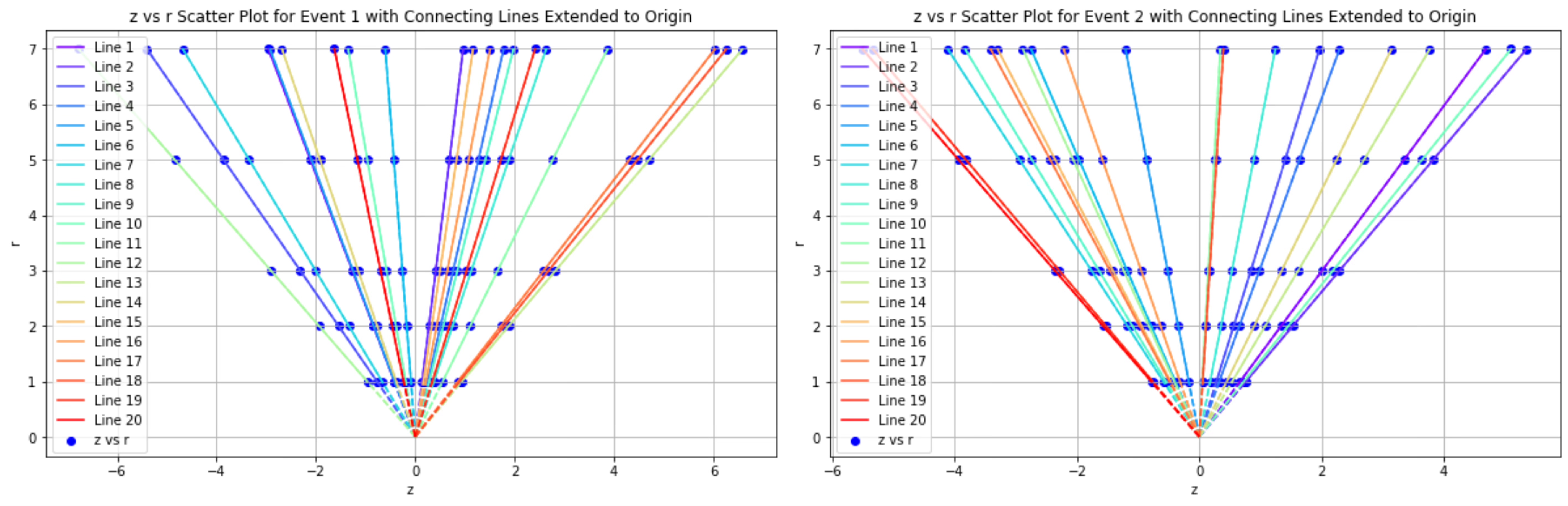
Figure 6. Flow chart of method in Track Finding

First establish the r-z coordinate system. Convert the x-y-z coordinates of the points into r-z coordinates and put them into the new coordinate system, then draw all the points [4]. These points are distributed on five layers, and we found that if these five points are a group, then they should form a straight line on the r-z plane and intersect at the origin. After that, through these two conditions, we match all five points on each trajectory in each event. (Figure 7 is an example of the two events in Track Finding.)

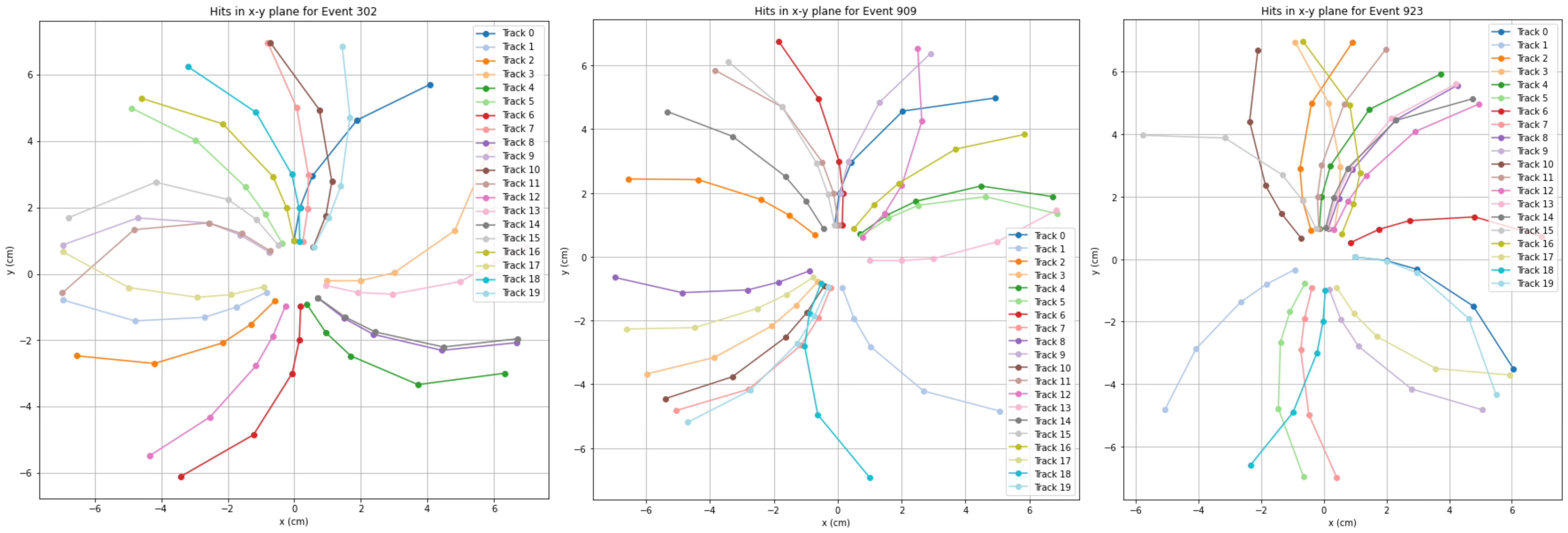
Figure 7. r-z Scatter Plot for the two events with Connecting Lines Extended to Origin

Second, put the points back into the x-y coordinate system and connect the lines. (Figure 8 is an example of three events in Track Finding.)

Figure 8. Hits and Tracks in x-y plane for random three events

Moreover, we make a mid-perpendicular line between the points in each set of five matched points. The point where the mid-perpendicular lines intersect is the center of the circular track. Next, connect the center of the circle and the point to get the radius R. The radius $$ r $$ of the circular track in the x-y plane can be calculated using the following formula:

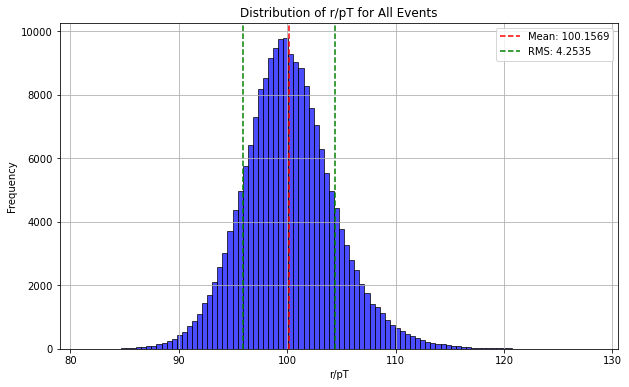
\begin{equation} r = \frac{1}{2} \sqrt{(x_2 - x_1)^2 + (y_2 - y_1)^2} \end{equation}

where $$ (x_1, y_1) $$ and $$ (x_2, y_2) $$ are the coordinates of two consecutive hits on the track. This formula determines the distance between two hit points, allowing for precise calculation of the track’s radius. By determining the radius, we can more accurately fit the particle’s trajectory [5]. We found all the tracks through determining the center and radius of each track. Then continue to calculate $$r/p_T(true)$$ for each event and to see if they are proportional. Because if the predicted circular track radius is correct, $$r/p_T(true)$$ should be proportional. Finally, Determine whether the radius of each circular track is correct by checking the distribution of $$r/p_T(true)$$ for all events. Then we found the distribution of $$r/p_T(true)$$ for all events that is centered around 100 with a standard deviation of around 4, which means all tracks are correct [6].

Figure 9. Distribution of $$r/p_T(true)$$ for All events

The method used in Track Fitting is that we designed a machine learning model. The machine learning model we have designed was based on predicting a transverse momentum ( $$p_T$$ ) related factor. Features are first extracted by fitting the initial hit points of each track into a circle. Subsequently, the actual points determined from the fitted circles were calculated, along with the average hit coordinates and momentum components. The baseline model pipeline started with the pre-processing step, where the features were standardized to have a mean of 0 and a variance of 1. Next, new interaction features were obtained via polynomial expansion. Using a Random Forest model, we were able to predict the target variable that represents the $$p_T$$ . The grid search was the method we used that was utilized for the optimization, which usually means the iterative approach with all data combinations. We also tried two models, MLP and XGboost, but we found the Random Forest model was the best [7]. Moreover, the performance of the optimized model was evaluated using cross-validation and on a separate test set. For that matter, R-squared score (the ratio of variance of explained variable explained by the model), and MSE (mean squared error), the average squared difference between actual values and predicted values - were selected as the key metrics. This way, we created a model with good predictive performance for a property of the particle system.

4. Experiments

The experiments were conducted to evaluate the effectiveness of our proposed methodology across the three main tasks: vertex finding, track finding, and track fitting. These tasks are critical for accurately determining the trajectory and momentum of particles in high-energy physics experiments.

4.1. Vertex Finding

In the vertex finding experiment, we started by visualizing the hits in the X-Y plane. By plotting these hits, we identified two distinct circles, corresponding to two layers of hits in the detector. We then connected corresponding points from the inner and outer =circles, filtered out any noise or erroneous points by checking distances, and extended these connections into the Z-plane to estimate the vertex location. The intersection points of these lines with the Z-axis were averaged to predict the Z-coordinate of the vertex. To achieve a more accurate vertex location, we use a weighted average formula to calculate the z-coordinate. By assigning a weight $$ w_i $$ to each hit based on its proximity to the actual vertex, we can reliably predict the vertex location:

\begin{equation} z_{vertex} = \frac{\sum_i w_i z_i}{\sum_i w_i} \end{equation}

where $$ z_i $$ is the z-coordinate of each hit and $$ w_i $$ is the corresponding weight. This weighted average method effectively reduces noise in the vertex prediction, improving the accuracy of the result [8]. This approach was repeated for each event in the dataset, leading to a robust prediction of the vertex location along the Z-axis.

4.2. Track Finding

For track finding, we first put the hit coordinates into an R-Z plane, where R is the radius in the X-Y plane. Then, We found the hits that correspond to the same track align into a straight line in this R-Z plane, which should ideally pass through the origin. After that, we grouped the hits into tracks each of them consist five points. After finding the correct tracks, we converted the coordinates back to the X-Y plane, where we performed a circular fit to determine the radius R for each track. Then we calculate r/ $$ p_T $$ to ensure our preciseness, where the predicted value is compared to the true values provided in the dataset, which ensures our predicted is near to the actual track and followed with real-life physical properties [9].

4.3. Track Fitting

Then, we focused on track fitting where we used the hits from the dataset to fit into a circular track. The elements used for track fitting included using radius R and. These features were then fed and put into different machine learning models to fit a circular path, including random forest regressor, MLP, and XGboost. The performance of these models is then evaluated by Mean Squared Error (MSE) and $$ R^2 $$ score. The dataset we used for our experiment comprised 10,000 events, each of which included 20 hits. The true vertex and tracking information were known, by making use of that, we can train our model and improve its accuracy, also ensure that our predicted output is close to the actual value. However, though some of the results are reasonable, some of the results from these experiments demonstrated the lack of robustness of our approach.

5. Results

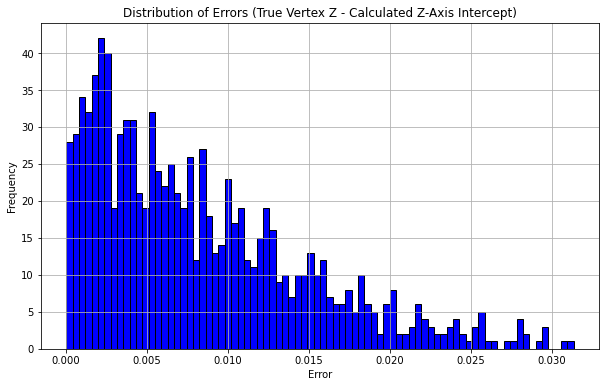
When it comes to vertex finding, after trying different parameters, improving the algorithm's robustness, and filtering the noises in the original data, we finally get a decent result. As we can see in the graph(Figure 10), we analyzed the error and got the distribution of the true vertex- calculated vertex. Our algorithm's mean error is 0.007999618, which is very close to 0 and precise.

Figure 10. The distribution of Error(True vertex - Predicted vertex)

When it comes to track finding, we also get satisfactory results. After trying different parameters and adding some filters to reduce the noise, we get precise data (Figure 11) compared to the true track (Figure 12). As we can see, the predicted track is very similar to the true track.

When it comes to track fitting, We tried different models, including MLP, random forest regressor, and XGBoost. By using MLP model, we obtained a MSE of 0.002, with an imprecise $$ R^2 $$ score of -2.472. In the track-fitting process, we calculate the residual to evaluate the accuracy of the fit. The residual is defined as:

\begin{equation} Residual = \sqrt{\sum_{i=1}^{n} (r_{fitted} - r_{true})^2} \end{equation}

The residual measures the error between the fitted track radius $r_{fitted}$ and the true track radius $r_{true}$ . A smaller residual indicates a more accurate fit. To evaluate the performance of the machine learning models, we use the MSE and the R-squared ( $$ R^2 $$ ) score, which are defined as follows:

\begin{equation} MSE = \frac{1}{n} \sum_{i=1}^{n} (y_{true, i} - y_{pred, i})^2 \end{equation}

\begin{equation} R^2 = 1 - \frac{\sum_{i=1}^{n} (y_{true, i} - y_{pred, i})^2}{\sum_{i=1}^{n} (y_{true, i} - \bar{y})^2} \end{equation}

The MSE measures the average squared difference between the predicted and actual values, while the $$ R^2 $$ score reflects how well the model fits the data. These metrics allow us to effectively evaluate the model’s performance in predicting the transverse momentum. Afterward, we used the XGBoost model, which produced a better result with an $$ R^2 $$ score of -0.806. We applied the random forest regressor to achieve better results, which provided reasonable outcomes. After training and finalizing our random forest regressor model, we achieved an MSE of 0.001, close to zero. However, the $$ R^2 $$ score still needs improvement, as it remained at -0.811 when using the same random forest regressor. Though we have a decent MSE, the poorness of the $$ R^2 $$ shows that our track-fitting model is not performing well in predicting the transverse momentum pT or accurately capturing the particle trajectories from the given data.

6. Conclusion and Discussion

In summary, this paper details a resilient technique to overcome the vertex retrieval, track identification, and track approximation problems that typically contest particle physics experiments. The strategy not only locates the vertices along the longitudinal axis with a high degree of accuracy but also tracks down the different tracks by the synergistic conjunction of hits, which sets the ground for precise momentum deductions. Following a process of circular fitting applied to the track data, the integration of radius and residuals into a machine-learning model eventually amplifies the predictive capacity of actual transverse momentum ( $$ p_T $$ ) by an order of magnitude. Through the use of a MLP model, random forest regressor, and XGboost for prediction, the agreement between predicted instead of actual $$ p_T $$ values is intended to improve, as well as to achieve a shrinkage in distribution and standard deviation. This all-including strategy not only enhances the accuracy of the trajectory and vertex evaluation but also outlines the opportunities of uniting conventional fitting techniques with cutting-edge machine learning in order to deepen the study of particle physics. The observations reveal the key roles of integrating advanced algorithms and models to extend the experimental accuracy and complexity in data analysis and interpretation.

References

[1]. De Cian, M., et al. (2012). Measurement of the track finding efficiency (No. LHCb-PUB-2011-025).

[2]. Lewis, R. (2020). Algorithms for finding shortest paths in networks with vertex transfer penalties. Algorithms, 13(11), 269.

[3]. Wang, Y., & Ma, J. (2021). Visual Object Tracking using Surface Fitting for Scale and Rotation Estimation. KSII Transactions on Internet & Information Systems, 15(5).

[4]. Shlomi, J., et al. (2021). Secondary vertex finding in jets with neural networks. The European Physical Journal C, 81(6), 1-12.

[5]. Jansen, B. M., et al. (2021). Vertex deletion parameterized by elimination distance and even less. In Proceedings of the 53rd Annual ACM SIGACT Symposium on Theory of Computing (pp. 1757-1769).

[6]. Lu, Z., Rathod, V., Votel, R., & Huang, J. (2020). Retinatrack: Online single stage joint detection and tracking. In Proceedings of the IEEE/CVF conference on computer vision and pattern recognition (pp. 14668-14678).

[7]. Peng, J., et al. (2020). Chained-tracker: Chaining paired attentive regression results for end-to-end joint multiple-object detection and tracking. In ECCV 2020 (pp. 145-161).

[8]. Zhou, X., Koltun, V., & Krahenb¨ uhl, P. (2020). Tracking objects as points. In European Conference¨ on Computer Vision (pp. 474-490). Cham: Springer.

[9]. Bols, E., Kieseler, J., Verzetti, M., Stoye, M., & Stakia, A. (2020). Jet flavour classification using DeepJet. Journal of Instrumentation, 15(12), P12012.

Cite this article

Chang,Y.;Wei,Z.;Cao,Q. (2025). Pattern Recognition and Prediction. Applied and Computational Engineering,132,241-249.

Data availability

The datasets used and/or analyzed during the current study will be available from the authors upon reasonable request.

Disclaimer/Publisher's Note

The statements, opinions and data contained in all publications are solely those of the individual author(s) and contributor(s) and not of EWA Publishing and/or the editor(s). EWA Publishing and/or the editor(s) disclaim responsibility for any injury to people or property resulting from any ideas, methods, instructions or products referred to in the content.

About volume

Volume title: Proceedings of the 2nd International Conference on Machine Learning and Automation

ISBN：978-1-83558-941-0(Print) / 978-1-83558-942-7(Online)

Editor：Mustafa ISTANBULLU

Conference website: https://2024.confmla.org/

Conference date: 21 November 2024

Series: Applied and Computational Engineering

Volume number: Vol.132

ISSN：2755-2721(Print) / 2755-273X(Online)

© 2024 by the author(s). Licensee EWA Publishing, Oxford, UK. This article is an open access article distributed under the terms and conditions of the Creative Commons Attribution (CC BY) license. Authors who publish this series agree to the following terms:
1. Authors retain copyright and grant the series right of first publication with the work simultaneously licensed under a Creative Commons Attribution License that allows others to share the work with an acknowledgment of the work's authorship and initial publication in this series.
2. Authors are able to enter into separate, additional contractual arrangements for the non-exclusive distribution of the series's published version of the work (e.g., post it to an institutional repository or publish it in a book), with an acknowledgment of its initial publication in this series.
3. Authors are permitted and encouraged to post their work online (e.g., in institutional repositories or on their website) prior to and during the submission process, as it can lead to productive exchanges, as well as earlier and greater citation of published work (See Open access policy for details).