1.Introduction

Generative models are models aim to produce a distribution that resembles the training data distribution or true distribution. The idea of generative models originated in the 1980s and its primary objective was to train models in an unsupervised way, reducing the amount of labor in collecting data for supervised learning [1]. Since then, generative models have developed and are performing exceptionally in producing high resolution, they have produced remarkable results in diverse realms of image processing. These achievements encompass image synthesis, modification, and even image classification [2]. Obtaining such successes relies on gaining representative features from the data, specifically in latent diffusion models, this involves extracting latent information of high-dimension data in lower-dimension spaces.

Before the diffusion models came along, Generative Adversarial Networks (GANs) and Variational Autoencoder (VAE) were the most popular image generation models, these two types of image generation models already obtained notable performance in generating realistic images [3]. The introduction of the diffusion model, a form of generative model that stems from Probabilistic Diffusion, has an enhanced ability to create more detailed and higher-quality images [3]. Later more developed models, e.g. latent diffusion model, incorporated autoencoders and conditional sampling techniques. This allowed the models to be less computationally expensive, in the meantime, the generation outputs were also more editable. The purpose of this paper is to assess different diffusion models and to analyze the results [4].

Since the advent of transformers (Vaswani, 2017), the field of machine learning, from natural language processing to computer vision, even reinforcement learning, have been revolutionized. The transformer model further enhanced the capability of feature extraction [5]. In 2023, Peebels and Xie constructed a new diffusion model incorporating the entire transformer block as its backbone, replacing the Unet construction [6]. This backbone sets the stage for later development in the diffusion model and gives the diffusion model better scaling ability. In this study, the author also compares this DiT model with LDM, the model DiT is based on. The contrastive language-image pre-training (CLIP) model is a multi-modality pretrained contrastive learning model that combines language training signal, or text signal, and vision signal to gain features of an image [7]. CLIP score is a score metric based on the CLIP model. This score is obtained by first acquiring a 512-D embedding from the image and the prompt generated the image, and then by using these embeddings for calculating a cosine similarity, this similarity value is the CLIP score [8]. This score aims to accurately depict the relationship between an image and the phrase that describes this image, the higher the cosine similarity is, the closer the relationship between the corresponding embedding pairs is.

This paper focuses on analyzing various diffusion models utilizing text-conditional sampling with the CLIP score as a metric. The CLIP model utilizes Bidirectional Transformers (BERT) and Vision Transformers (ViT) to extract text and image embeddings from image captions and the images themselves [9][10]. As the CLIP model is closely tied to transformer architecture, it's crucial to compare diffusion models that incorporate transformer blocks with those that do not use transformers as decoders. This study focuses on comparing the structures of latent diffusion models and diffusion transformer models. The former employs a Unet decoder, while the latter integrates a Transformer block as its decoder. Additionally, this study explores various prompts aimed at generating similar images, seeking suitable forms of textual cues to aid in training diffusion models with text-to-image generation capabilities and to inform future research endeavors.

2.Methodology

2.1.Dataset and Preprocessing

This study focused on four image datasets, Cifar10, Cifar100, and ImageNet [11][12]. Cifar10 and Cifar100 both are created by Alex Krizhevsky, et al. Each of the Cifar10 and Cifar100 datasets contains 60,000 labeled colored images with size of 32×32. Cifar10 and Cifar100, as their names suggest, are composed of 10 categories of pictures and 100 categories of pictures respectively. ImageNet was introduced by Jia Deng et al in 2009. There are different types of ImageNet datasets, they are all made for non-commercial use. The most commonly used ImageNet dataset is ImageNet10K, a dataset with 1000 classes that contains over 1.2 million colored images with varying sizes. MNIST was introduced in 1998 by Yann LeCun, it is a dataset containing 70000 handwritten images for the 10 digits, 60000 for training, and 10000 for testing. They are all in grayscale and with the size of 28×28. These datasets have simple labels for each image, this paper uses the images’ class labels as base-prompts to generate images. On top of that, this study gradually adds in different levels of details to the class label for image generation to compare CLIP scores.

2.2.Architecture

This paper examines the accuracy of the CLIP score when using DiT and latent diffusion models for image generation. Since the DiT model lacks a pretrained text conditioning model, the author employed the class names from the ImageNet dataset as image prompts. The study generated 500 images in total, with 5 images per class for 10 to 100 classes simultaneously. To manage the vast

number of ImageNet classes, the author randomly selected 100 classes for image generation. After generating the images using latent diffusion and DiT models, they standardized the image sizes to 224 × 224 pixels. Subsequently, both the images and their corresponding description texts underwent processing through ViT and text transformers to obtain embeddings. These embeddings were normalized and utilized to compute an averaged cosine similarity for subsequent analysis. The pipeline is depicted in figure 1. The text prompt is the input of text to image generation model, or the it is the name of the image class (in DiT). Then it goes through the text transformer to get the embedding. The generated image goes through ViT/14 to get an embedding. At the end, the embeddings are normalized and embeddings in the same class are used to gain an average cosine similarity.

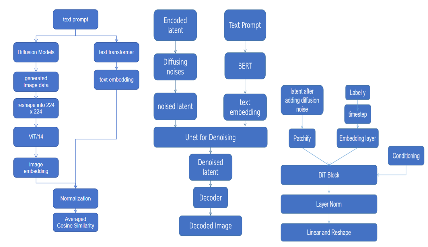
Figure 1: Pipeline for the evaluation, LDM and DiT (Photo/Picture credit: Original)

2.2.1.Variational Autoencoder (VAE)

The VAE is the first step for both the latent diffusion model and the Diffusion Transformer model. This VAE model assumes the image dataset\( X \)consists of n-many i.i.d data\( {x_{i}}, i = 1, ..., n. \)The encoder\( E({x_{i}}) \)of VAE tries to acquire latent representation\( {z_{i}} \) for each\( {x_{i}} \), the docoder\( D(z) \)tries to predict the image from a given latent\( z \). Specifically in the latent diffusion model, the input\( x \)is an image with size of\( H × W × 3 \), and\( z \)is a latent of the image z with dimension of\( h × w× c \), smaller than image\( x \)by a downsampling factor\( f = \frac{H}{h}= \frac{W}{w} \), here\( f = {2^{m}} \) for some\( m ∈N \). In comparison to a 1-dimensional latent in some works of the LDM paper’s authors, this\( z \)has a 2-dimensional structure, this is an attempt to retain more information from the original image [4]. The diffusion model uses a VAE with KL-regularization, after extracting the latent\( z \)using VAE, the representation\( z \)then goes into the diffusion process.

2.2.2.Denoising Diffusion Probailistic Models (DDPMs)

The Diffusion process consists of 2 stages, a noise-adding forward process and a reverse process for denoising. Both of these processes are Markov chains. The forward process progressively diffuses Gaussian noise into the input image, while the reverse process removes the noise to acquire an image.

In the Forward process, the DDPM grabs an image data x₀ from the given dataset. Assume there are\( T \)many timesteps in the forward process, in a certain timestep\( t \), such that\( 1 ≤ t ≤ T \), the noised image data\( {x_{t}} \)is obtained as shown in the following formula:

\( {x_{t}} = {{(\bar{α}_{t}})^{\frac{1}{2}}}{x_{0}}+ {(1-{\bar{α}_{t}}ϵ)^{\frac{1}{2}}} \)(1)

where\( ϵ \)is a Gaussian noise with the same dimension as\( x \),\( {α_{t}} \) is a scaling factor indicating at given time step\( t \), what portion of sampled Gaussian noise is added to the original image\( x \).\( {α_{t}} := 1 - {β_{t}} \), where\( {β_{t}} \)is a variance schedule that increases as\( t \)increases from\( 1 \)to\( T \). At time step\( T \), the original image\( {x_{0}} \)is fully converted to a Gaussian noise\( {x_{T}} \).

The Reverse process is autoregressive, it slowly reduces the noise from the Gaussian noise\( {x_{T}} \)to reconstruct the original image. The Sampling process focuses on the reverse process, it uses a predicted noise\( {ϵ_{θ}} \), a noise\( z \)sampled from N (0,1), given the timestep\( t \), the clearer image in the next reverse timestep\( t-1 \)is given as:

\( {x_{t-1}}= {{(\bar{α}_{t}})^{-\frac{1}{2}}} ({x_{t}}-{(\frac{1 - {α_{t}}}{ {(1-{\bar{α}_{t}}ϵ)^{\frac{1}{2}}}})ϵ_{θ}}({x_{t}},t))+{σ_{t}}z \)(2)

where\( {σ_{t}}I= {Σ_{θ}}({x_{t}}, t) \)is the covariance matrix of the conditional probability distribution\( {p_{θ}}({x_{t-1}}|{x_{t}}) := \)N\( ({x_{t-1}};{μ_{θ}}({x_{t}},t),{Σ_{θ}}({x_{t}}, t)) \)

2.2.3.DiT Block

The diffusion transformer block (DiT) is a replacement for the Unet structure to improve the scalability of the latent diffusion model. This block is based on the ViT architecture, it uses patches to extract information from the image latent in the patchify layer, which is also the first layer of the DiT model. In this layer, it turns the latent of the noised image, with the size of\( I × I × C \)to an input token with length\( T \)and dimension\( d \). Where\( T = {(\frac{I}{p})^{2}} \), and\( p \)is the length of one patch, each image can be breakdown into T many patches. After patchifying, input token and the conditioning will be passed to the DiT block. There are four types of DiT blocks, the one that has the best FID-50K performance is the block called the adaLN-Zero block. Such type of DiT block combines adaptive normalization layer and a zero-initialization in the final convolutional layer in the DiT block, after this, the DiT block then goes into the residual connection process.

2.2.4.CLIP Score

CLIP Score utilized the CLIP model. In this paper, ViT model is used to obtain image embeddings and text transfomrer is used to obtain text embeddings in the CLIP model. 5 images or 10 images are generated from the same class and a total of the embeddings are normalized to the interval [0, 1], these embeddings is then evaluated with all the text prompts that used to generate the images or those that describe the images, using the cosine similarity. The similarity values are averaged between all the images in the same class. For example, if each class has 5 images, the mean of the 5 similarity values will be the final average score for this class. Comparisons of CLIP Scores. In this paper, LDM is pretrained by using the LAION5B dataset and DiT model is pretrained by using ImageNet dataset. This paper compares the CLIP Scores for the generated images and the images from the original dataset by using these two models.

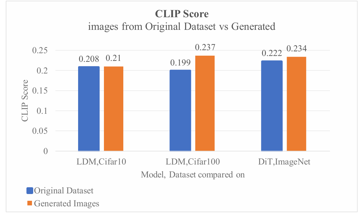
Figure 2: The CLIP score (Photo/Picture credit: Original)

3.Results and Discussion

In order to evaluate the behavior of the CLIP score relating to the description sentence in this study, the author finds CLIP scores using various types of prompts. First, the author evaluates the CLIP Scores between the pictures of the datasets with the class labels. In addition, the author kept the default setting of the CLIP model, adding a “This is” phrase in front of the class label. For example, in the Cifar100 dataset, the prompts look like “This is aquatic mammal beaver”, in the Cifar10 dataset, the prompts look like “This is airplane”. Second, the CLIP score is generated by calculating the generated graph of the diffusion model and the text of the generated picture, or the name of its corresponding category.

As Shown in figure 2 the images Cifar10 dataset and the ImageNet dataset have similar CLIP Scores with the generated images. However, there is a large difference between the CLIP Scores of the Cifar100 dataset and the generated images. A possible reason for this is the classifier prompts for the Cifar100 are formed by combining the superclass labels and the specific class labels. As mentioned before, the Cifar100 dataset’s labels look like “aquatic mammal beaver”, and the Cifar10 dataset’s class labels look like “airplane”. This is shown in figure 3, with the removal of the superclass labels in Cifar100, the CLIP Score decreases by 13% of the original Score. Two causes could lead to such a result. First, the difference between prompts that generated the image and the prompts that removed the superclass names are now different. Second, the prompts without superclass names now have reduced relevant information than the original prompt. Comparison of CLIP Scores between prompts that used superclass and those without superclass added.

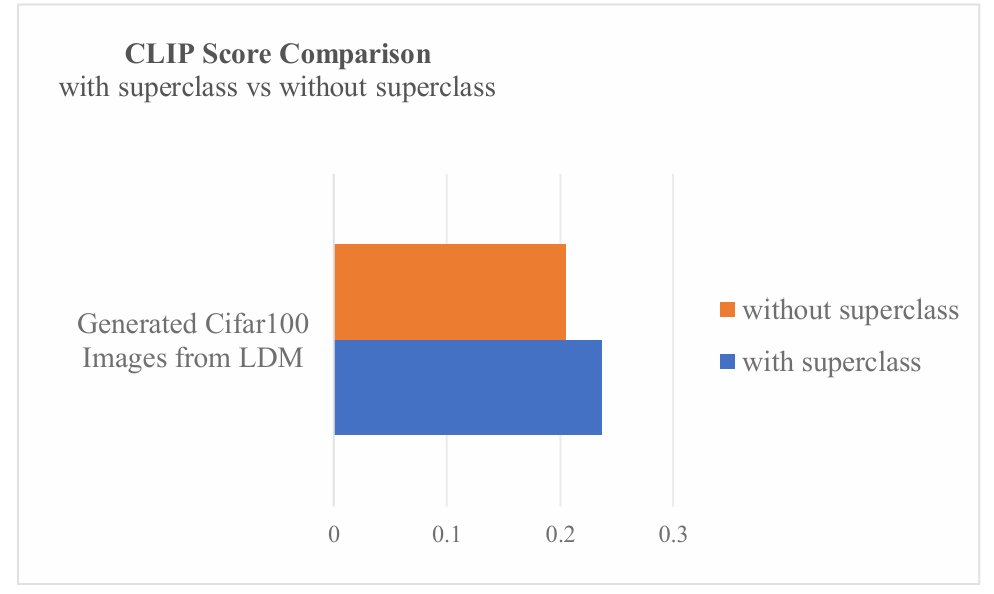
Figure 3: The comparison of CLIP score (Photo/Picture credit: Original)

4.Conclusion

This study evaluates the performance of the LDM and the DiT model, alongside examining the impact of prompt structure on the CLIP Score. Given that LDM utilizes text embeddings based on the CLIP model, investigating how generative models interact with these embeddings offers insights into enhancing the conditioning training process. Comparisons of CLIP scores are made between original dataset images and those generated by diffusion models. Initially, CLIP scores are calculated against the class names of images in all datasets. Subsequently, superclass names are excluded from prompts in the Cifar100 dataset for further CLIP score calculations. The findings reveal higher CLIP scores for generated images across all datasets, particularly evident when comparing Cifar100 dataset images with those generated using Cifar100 class names as prompts. Further analysis indicates a decrease in CLIP scores upon the removal of superclass prompts. While time constraints limited additional comparisons, future research will explore the performance of the multimodal DiT model, combining CLIP with DiT, and assess CLIP scores for various prompt structures in text conditioning DiT models. Additionally, the investigation into the disparities in CLIP scores for LDM models concerning the Cifar100 dataset is planned.

References

[1]. Li A. C, Prabhudesai, M., Duggal, S., Brown, E., & Pathak, D. (2023). Your diffusion model is secretly a zero-shot classifier. In Proceedings of the IEEE/CVF International Conference on Computer Vision (pp. 2206-2217).
[2]. Bond-Taylor S, Leach A, Long Y, & Willcocks C. G. (2021). Deep generative modelling: A comparative review of vaes, gans, normalizing flows, energy-based and autoregressive models. IEEE transactions on pattern analysis and machine intelligence, 44(11), 7327-7347.
[3]. Ho J, Jain A, & Abbeel P. (2020). Denoising diffusion probabilistic models. Advances in neural information processing systems, 33, 6840-6851.
[4]. Rombach R, Blattmann A, Lorenz D, Esser P, & Ommer B. (2022). High-resolution image synthesis with latent diffusion models. In Proceedings of the IEEE/CVF conference on computer vision and pattern recognition (pp. 10684-10695).
[5]. Vaswani A, Shazeer N, Parmar N, Uszkoreit J, Jones L, Gomez A. N, ... & Polosukhin I (2017). Attention is all you need. Advances in neural information processing systems, 30.
[6]. Peebles W, & Xie S (2023). Scalable diffusion models with transformers. In Proceedings of the IEEE/CVF International Conference on Computer Vision (pp. 4195-4205).
[7]. Radford A, Kim J. W, Hallacy C, Ramesh A, Goh G, Agarwal S, ... & Sutskever I. (2021, July). Learning transferable visual models from natural language supervision. In International conference on machine learning (pp. 8748-8763). PMLR.
[8]. Hessel J, Holtzman A, Forbes M, Bras R. L, & Choi Y (2021). Clipscore: A reference-free evaluation metric for image captioning. arXiv preprint arXiv:2104.08718.
[9]. Devlin J, Chang M. W, Lee K, & Toutanova K (2018). Bert: Pre-training of deep bidirectional transformers for language understanding. arXiv preprint arXiv:1810.04805.
[10]. Dosovitskiy A, Beyer L, Kolesnikov A, Weissenborn D, Zhai X, Unterthiner T, ... & Houlsby N (2020). An image is worth 16x16 words: Transformers for image recognition at scale. arXiv preprint arXiv:2010.11929.
[11]. Krizhevsky A, & Hinton G (2009). Learning multiple layers of features from tiny images.
[12]. Deng J, Dong W, Socher R, Li L. J, Li K, & Li F (2009, June). Imagenet: A large-scale hierarchical image database. In 2009 IEEE conference on computer vision and pattern recognition (pp. 248-255). Ieee.
Cite this article
Tang,Q. (2025). Analyzing Diffusion Models: Transformer Integration and Prompt Optimization for Text-To-Image Generation. Applied and Computational Engineering,108,175-181.
Data availability
The datasets used and/or analyzed during the current study will be available from the authors upon reasonable request.
Disclaimer/Publisher's Note
The statements, opinions and data contained in all publications are solely those of the individual author(s) and contributor(s) and not of EWA Publishing and/or the editor(s). EWA Publishing and/or the editor(s) disclaim responsibility for any injury to people or property resulting from any ideas, methods, instructions or products referred to in the content.
About volume
Volume title: Proceedings of the 5th International Conference on Signal Processing and Machine Learning
© 2024 by the author(s). Licensee EWA Publishing, Oxford, UK. This article is an open access article distributed under the terms and
conditions of the Creative Commons Attribution (CC BY) license. Authors who
publish this series agree to the following terms:
1. Authors retain copyright and grant the series right of first publication with the work simultaneously licensed under a Creative Commons
Attribution License that allows others to share the work with an acknowledgment of the work's authorship and initial publication in this
series.
2. Authors are able to enter into separate, additional contractual arrangements for the non-exclusive distribution of the series's published
version of the work (e.g., post it to an institutional repository or publish it in a book), with an acknowledgment of its initial
publication in this series.
3. Authors are permitted and encouraged to post their work online (e.g., in institutional repositories or on their website) prior to and
during the submission process, as it can lead to productive exchanges, as well as earlier and greater citation of published work (See
Open access policy for details).