1. Introduction

With the development of robotics, robots are widely used in manufacturing, medical, rescue and other fields. As an emerging robotics, it has high dexterity compared to continuum robots. This flexibility gives continuum robots a unique advantage in confined spaces. Thus, continuum robot research has become a major area of current research [1].

Due to the simplicity of the method, tendon drive mechanism is one of the frequently used drive methods for continuum robots [2]. Tendon-driven continuum robots (TDCRs) are composed of a driving tendon, a flexible backbone, disks, and other devices [3]. Modeling of the TDCRs is challenging, which are increased by continuum robots having almost infinite degrees of freedom. [4]. Kinematic models have been applied widely in the modeling process of continuum robots. The constant curvature model assumes that the robot has a defined geometry. [1]. Geometric models are one of the most common models used in soft robotics research. TDCR motions are divided into multiple circular arcs by it.

The solution of workspace is very important for the control of continuum robot [5]. The workspace, serving as a performance indicator for continuum robots, establishes the robot's application and functions. However, the number of continuum robot segments may vary depending on the size and shape of the workspace.

Currently, there is a gap in the area of the impact of the number of segments of a continuum robot on the workspace. Many researchers work with continuum robots that have a specific number of segments. The kinematic modeling of two-segment continuum robot is studied in reference I, and the kinematic modeling of single-segment continuum robot is studied in Reference II [1].[2]. This research on the effect of the number of continuum robots can help in the selection of a more appropriate number of segments, thereby contributing to the construction of more efficient continuum robots. Therefore, it is crucial to study the range of the number of segments of the continuum robots.

In this work, we investigate the workspace of a single-segment continuum robot and also a two-segment continuum robot. Firstly, a single-segment robot and a two-segment robot are modeled by the segmented constant curvature method. Next, Peter I. Corke proposed a method for determining kinematic parameters using the DH convention [6]. we need to conduct a kinematic analysis of continuum robots using the DH method, which establishes a coordinate system and creates relationships between the workspace to control the real-time shape. We have derived the corresponding kinematic equations for continuum robots.

In recent years, the Monte Carlo method has widely used in the construction of the workspace. Granna, J., and Burgner, J. used the Monte Carlo method to solve for the workspace of a concentric tube continuum robot[7]. This method uses random sampling to obtain numerical results. It provides a reliable statistical estimate of the volume of the workspace. Therefore, Monte Carlo method is used to address the workspace of TDCR in this work. The core contributions are listed as follows:

• We used a constant curvature model to describe the attitude of each segment in detail. A coordinate system was developed using the D-H method to express the end positions This provides the basis for further workspace analysis.

• We compared the workspace of a single-segment continuum robot with that of a two-segment continuum robot. By comparing the workspace volumes drawn by the two configurations, we demonstrate the effect of the number of segments on the workspace. This study offers a rationale for the selection process.

The remaining parts of this paper are organized as follows. Section II describes the relevant work. Section III derives the kinematic modeling of a tendon-driven continuum robot. Section IV describes the simulation workflow of the workspace. Section V concludes the paper by considering future avenues of development, such as further exploration of the impact of segment numbers on workspace, and the potential application of our findings in the design and control of TDCRs.

2. Related Work

In recent years, as robotics has advanced rapidly, a new type of soft robot, due to its structural flexibility and high degree of freedom, has been used in various applications, such as medical care. The prototype of continuum robots appeared in the 1960s, and related research was carried out in the 1980s. Robinson and Davies et al. 1999 presented the basic concept of continuum robots [8]. Continuum robots are defined as a class of robots whose structure bends through elastic deformation to achieve a state of curvilinear motion similar to that of a tentacle. Related research has studied bionic continuum robots, such as octopus tentacles and elephant trunks [3, 9].

There have been many approaches to modeling continuum robots [1]. The constant curvature model is the most common way to model continuum robots because it is easy to understand. It is also widely used to make geometric and kinematic analysis of robots easier. Fig. 1 is a diagram of the relationship between the three spaces and their mappings in the TDCRs. The constant curvature model, is one of the key approaches for the kinematic modeling of the TDCR, which characterizes the shape of each segment as a circular arc of constant length. The application of constant curvature models can simplify the model, which is important for simplifying the modelling of complex models.

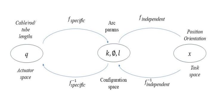
Figure 1: Three spaces and their mapping relationships of the TDCR

Numerous scholars have used the constant curvature model in the study of continuum robots. The DH parametric method is commonly used in robot kinematic modeling, which is mainly used to describe the kinematic relationships of multi-degree-of-freedom robots. Denavit and Hartenberg first proposed this method, which is only applicable to rigid robots [10]. Later, other scholars applied the DH parametric method to the field of continuum robots through further research and exploration. Recently, Jones and Walker looked into how the DH method can be used to model the motion of multi-segment continuum robots and how to use the DH method in multi-segment continuum robot models [2]. Zhao and Zhang also proposed the application of the DH method in modeling continuum robots, focusing on how to improve the workspace of the robot by optimizing the DH parameters [11]. Guidance on selecting TDCR models can help the user choose the right model based on the trade-offs between accuracy and calculation time required for different design parameters. This has important implications for the control of TDCRs [12].

Robotic systems widely use Monte Carlo methods to compute workspace. The Monte Carlo methods utilizes random sampling to simulate the workspace by simulating a large number of random samples. As the number of samples increases, the closer the experimental results are to the real values [13].

3. Kinematic Modeling of TDCR

This model is based on the assumption that the TDCR segment's curvature (κ) keeps the same while it bends. The curvature κ, the rotation angle φ, and the segment length l are used to describe the segment's attitude.

For kinematic modeling of a TDCR, we start by using the local transformation matrix T to find out where each segment is in its own set of coordinates. In Eq. (1), we begin with the definition of the transformation matrix. It denotes rotation about the z-axis, denotes rotation about the y-axis, and is the translation variable.

\( T=\underset{Rotation }{\underbrace{[\begin{matrix}{R_{z}}(ϕ) & 0 \\ 0 & 1 \\ \end{matrix}]}}\underset{Inplane transformation }{\underbrace{[\begin{matrix}{R_{y}}(θ) & p \\ 0 & 1 \\ \end{matrix}]}} \) (1)

This matrix combines rotations and translations and is used to calculate the position and orientation of the end of the robot segment in the local coordinate system. The matrix in Eq. (2) describes the transformation of the robot segment from the local frame to global frame, including changes due to curvature κ and rotation angle ϕ. The application of Eq. (2) can be directly applied to find the workspace of a single-segment continuum robot.

\( {T_{1}}=[\begin{matrix}cos⁡{ϕ_{1}}cos⁡{κ_{1}}{s_{1}} & -sin⁡{ϕ_{1}} & cos⁡{ϕ_{1}}sin⁡{κ_{1}}{s_{1}} & \frac{cos⁡{ϕ_{1}}(1-cos⁡{κ_{1}}{s_{1}})}{{κ_{1}}} \\ sin⁡{ϕ_{1}}cos⁡{κ_{1}}{s_{1}} & cos⁡{ϕ_{1}} & sin⁡{ϕ_{1}}sin⁡{κ_{1}}{s_{1}} & \frac{sin⁡{ϕ_{1}}(1-cos⁡{κ_{1}}{s_{1}})}{{κ_{1}}} \\ -sin⁡{κ_{1}}{s_{1}} & 0 & cos{κ_{1}}{s_{1}} & \frac{sin⁡{κ_{1}} {s_{1}}}{{κ_{1}}} \\ 0 & 0 & 0 & 1 \\ \end{matrix}] \) (2)

Two-segment continuum robot workspace solved by representing the global position of the second segment. Firstly, the end position of the first segment can be expressed by Eq.(2). we solve for the local variation matrix of the second segment \( { T_{2,local}} \) . \( {T_{2,local}} \) contains the curvature \( {κ_{2}} \) ​ of the first segment, the direction of curvature \( {ϕ_{2}} \) , and the length of the segment \( {l_{2}} \) , of which Eq. (3) is as follows.

\( {T_{2,local}}=[\begin{matrix}cos⁡{ϕ_{2}}cos⁡{κ_{2}}{s_{2}} & -sin⁡{ϕ_{2}} & cos⁡{ϕ_{2}}sin⁡{κ_{2}}{s_{2}} & \frac{cos⁡{ϕ_{2}}(1-cos⁡{κ_{2}}{s_{2}})}{{κ_{2}}} \\ sin⁡{ϕ_{2}}cos⁡{κ_{2}}{s_{2}} & cos⁡{ϕ_{2}} & sin⁡{ϕ_{2}}sin⁡{κ_{2}}{s_{2}} & \frac{sin⁡{ϕ_{2}}(1-cos⁡{κ_{2}}{s_{2}})}{{κ_{2}}} \\ -sin⁡{κ_{2}}{s_{2}} & 0 & cos{κ_{2}}{s_{2}} & \frac{sin⁡{κ_{2}} {s_{2}}}{{κ_{2}}} \\ 0 & 0 & 0 & 1 \\ \end{matrix}] \) (3)

Eq. (4) is used to solve for the workspace of a two-segment continuum robot. \( {T_{global}} \) denotes the two-segment continuum robot end workspace. It is solved by multiplying the end transformation matrix \( {T_{1}} \) of the first segment with the local transformation matrix \( {T_{2,local}} \) of the second segment. The procedure is shown in Eq. (4)

\( {T_{global}}={T_{1}}∙{T_{2,local}} \) (4)

4. Simulation

We have developed a program containing a kinematic model of TDCRs and the associated MATLAB code for the Monte Carlo method of finding the workspace. Implemented in MATLAB on a laptop computer with a 12th generation Intel(R) Core(TM) i5-12500H, 2500 Mhz, 12 cores, 16 logical processors running the Windows operating system. We evaluate workspaces primarily in terms of their volume.

In the simulation of a single-segment continuum robot, the input parameters are the following, including the rope length variation range of ±0.01 m, the length of a single base segment l of 0.2 m long, the number of disks per segment n = 10 and the radius of the disk \( {R_{risk}} \) = \( 10×{10^{-3}} \) m.

We calculate the workspace volume according to Eq. (5) \( {; l_{1}},{l_{2}},{ and l_{3}} \) represent the three rope lengths of a single segment, respectively. With respect to finding the workspace, we use the Monte Carlo method. Generated 100,000 random samples within the rope activity area. After generating the random points, Eq. (4) is used to solve for the end positions of the random samples. The end positions of each sample are then solved, and these positions are formed into a point cloud for output. Subsequently, the convex packet algorithm is applied to the point cloud to obtain the output parameters, i.e., the volume \( {V_{1}} \) ​ of the workspace is estimated.

For the simulation of a two-segment continuum robot, input parameters include rope length variation range ±0.01m, the length of a single base segment l of 0.2 m long, the number of disks per segment n = 10 and the radius of the disk \( {R_{risk}} \) = \( 10×{10^{-3}}m \) .

The calculation of the workspace volume \( {V_{2}} \) is based on the Eq. (6) In the equation, \( {l_{1}},{l_{2}},{l_{3}} \) are the lengths of the ropes in the first section, while \( {l_{4}},{l_{5}},{l_{6}} \) are the lengths of the ropes in the second section. Simulation based on the Monte Carlo method to generate 100000 random samples and calculate the end position corresponding to each random sample. After generating the random points, Eq. (4) is used to solve for the end positions of the random samples. The point cloud uses the convex packet algorithm to estimate the workspace volume and get the output parameter \( {V_{2}} \) .

\( {V_{1}}={F_{1}}({l_{1}},{l_{2}},{l_{3}}) \) (5)

\( { V_{2}}={F_{2}}({l_{1}},{l_{2}},{l_{3}},{l_{4}},{l_{5}},{l_{6}}) \) (6)

5. Results and Discussion

The results are analysed in this section.Fig.2 showed the workspace of a single-segment continuum robots. As can be seen from the figure, the workspace exhibited an ellipsoidal structure resembling an incomplete, the extension in the Z-axis direction was limited. This single-segment robot has limited movement capabilities, Demonstrating the limited manipulation capability of a single-segment robot.

Fig. 3 shows the results of the calculation of the point cloud volume in the workspace of a single-segment continuum robot, with volume \( {V_{1}}=0.0012847{m^{3}} \)

.

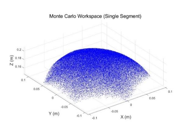
Figure 2: Monte Carlo method for the workspace of single-segment continuum robots.

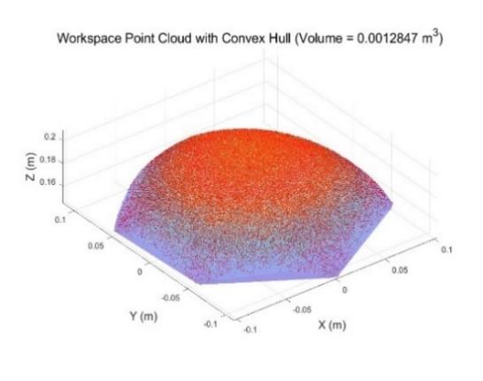
Figure 3: Volume of workspace for single-segment continuum robots

Fig. 4 illustrates the workspace of a two-segment continuum of robots. Compared to single-segment robots. The workspace of the two-segmented robot expanded in all three dimensions, forming a larger and more complete ellipsoidal structure. This showed that the dual-segment design significantly improves robot coverage.

Fig. 5 shows the results of the calculation of the point cloud volume in the workspace of the two-segment continuum robots with volume \( {V_{2}}=0.060067{m^{3}} \) .

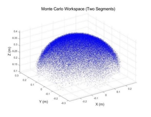
Figure 4: Monte Carlo method for the workspace of two-segment continuum robots

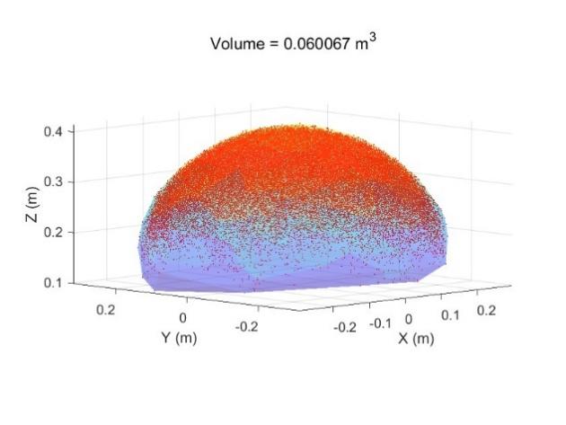
Figure 5: The volume of workspace for two-segment continuum robots

6. Conclusion and Future Work

In this research, the workspace characteristics of single-segment and two-segment continuum robots were comprehensively analyzed using Monte Carlo simulation methods.

The results demonstrate that the volume of the workspace for a two-segment continuum robot is not linearly proportional to the volume of the workspace of a single-segment continuum robot. Specifically, two-segment continuum robots exhibit a substantially larger workspace compared to single-segment continuum robots. The geometry of the workspace for the two-segment continuum robot tends to be more ellipsoidal, in contrast to the shape of the workspace associated with the single-segment continuum robot. The movement range of the single-segment continuum robot is notably restricted in the Z-axis direction. Therefore, the two-segment continuum robot offers a broader scope of motion and a higher degree of flexibility.

Dynamic modelling of continuum robots in changing environments can enhance the accuracy of robots in rapid movement. In this research, the effects of gravity and friction on the workspace in practical applications are not considered. Thus, a deeper effect of the number of segments on the continuum robots can be determined. Future work will focus on the workspace analysis based on the dynamic model.

References

[1]. Webster III, R. J., & Jones, B. A. (2010). Design and kinematic modeling of constant curvature continuum robots: A review. The International Journal of Robotics Research, 29(13), 1661-1683.
[2]. Jones, B. A., & Walker, I. D. (2006). Kinematics for multisection continuum robots. IEEE Transactions on Robotics, 22(1), 43-55.
[3]. Laschi, C., Cianchetti, M., Mazzolai, B., Margheri, L., Follador, M., & Dario, P. (2012). Soft robot arm inspired by the octopus. Advanced robotics, 26(7), 709-727.
[4]. Rao, P., Peyron, Q., Lilge, S., & Burgner-Kahrs, J. (2021). How to model tendon-driven continuum robots and benchmark modelling performance. Frontiers in Robotics and AI, 7, 630245.
[5]. Mason, M. T. (2001). Mechanics of robotic manipulation. MIT press.
[6]. Granna, J., & Burgner, J. (2014, June). Characterizing the workspace of concentric tube continuum robots. In ISR/Robotik 2014; 41st International Symposium on Robotics (pp. 1-7). VDE.
[7]. Corke, P. I. (2007). A simple and systematic approach to assigning Denavit–Hartenberg parameters. IEEE transactions on robotics, 23(3), 590-594.
[8]. Robinson, G., & Davies, J. B. C. (1999, May). Continuum robots-a state of the art. In Proceedings 1999 IEEE international conference on robotics and automation (Cat. No. 99CH36288C) (Vol. 4, pp. 2849-2854). IEEE.
[9]. Ma, K., Chen, X., Zhang, J., Xie, Z., Wu, J., & Zhang, J. (2023). Inspired by physical intelligence of an elephant trunk: Biomimetic soft robot with pre-programmable localized stiffness. IEEE Robotics and Automation Letters, 8(5), 2898-2905.
[10]. Denavit, J., & Hartenberg, R. S. (1955). A kinematic notation for lower-pair mechanisms based on matrices.
[11]. Cao, K., Kang, R., Branson III, D. T., Geng, S., Song, Z., & Dai, J. S. (2017). Workspace analysis of tendon-driven continuum robots based on mechanical interference identification. Journal of Mechanical Design, 139(6), 062303.
[12]. Rao, P., Peyron, Q., Lilge, S., & Burgner-Kahrs, J. (2021). How to model tendon-driven continuum robots and benchmark modelling performance. Frontiers in Robotics and AI, 7, 630245.
[13]. Metropolis, N., & Ulam, S. (1949). The Monte Carlo method. Journal of the American Statistical Association, 44(247), 335-341.
Cite this article
Wang,Y. (2025). Workspace Analysis of the Tendon-driven Continuum Robots with Different Numbers of Segments. Applied and Computational Engineering,134,10-16.
Data availability
The datasets used and/or analyzed during the current study will be available from the authors upon reasonable request.
Disclaimer/Publisher's Note
The statements, opinions and data contained in all publications are solely those of the individual author(s) and contributor(s) and not of EWA Publishing and/or the editor(s). EWA Publishing and/or the editor(s) disclaim responsibility for any injury to people or property resulting from any ideas, methods, instructions or products referred to in the content.
About volume
Volume title: Proceedings of the 5th International Conference on Signal Processing and Machine Learning
© 2024 by the author(s). Licensee EWA Publishing, Oxford, UK. This article is an open access article distributed under the terms and
conditions of the Creative Commons Attribution (CC BY) license. Authors who
publish this series agree to the following terms:
1. Authors retain copyright and grant the series right of first publication with the work simultaneously licensed under a Creative Commons
Attribution License that allows others to share the work with an acknowledgment of the work's authorship and initial publication in this
series.
2. Authors are able to enter into separate, additional contractual arrangements for the non-exclusive distribution of the series's published
version of the work (e.g., post it to an institutional repository or publish it in a book), with an acknowledgment of its initial
publication in this series.
3. Authors are permitted and encouraged to post their work online (e.g., in institutional repositories or on their website) prior to and
during the submission process, as it can lead to productive exchanges, as well as earlier and greater citation of published work (See
Open access policy for details).