


1. Introduction
Digital cameras have become the most commonly used devices for image perception. A charge-coupled device (CCD), which functions as a sensor and enables the capture of colourful still images, can be viewed as a key component of a digital camera. RGB(red, green, and blue), also referred to as the "three primary colours", can be combined to create any visible colour of light . As a result, conventional CCD uses a Bayer mosaic pattern, with each set of pixels having two green filters that are arranged diagonally, one red filter, and one blue filter [1]. Although the development of CCD significantly decreased the cost and improved the convenience of taking pictures, a large number of mosaics will be produced in the captured images [2].
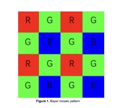
In addition to the hardware improvement of improving the image quality, the research on the algorithm can also greatly improve the image resolution. Although some old algorithms are relatively simple and only have a small amount of calculation, the capacity to obtain the pixels that surround the points are poor, so the image quality may not be perfect. The advanced algorithm has its progress, but there are still has its shortcomings. As seen in Fig. 1, the design of CCD leaves each pixel with only one precise colour single channel value, necessitating the determination of values of the other two channel colours.
|
Figure 1. Bayer mosaic pattern. |
There would be a lot of mosaic on the processed image if the interpolation algorithm was ineffective. There are many algorithms are suggested to get rid of mosaic. By using the RGB values of its closest neighbours, it is possible to hypothesize the missed RGB value of a single pixel. Given there are a lot of proposed algorithms, there are two common problems when processing the images. One of them is false colouring. This effect is most noticeable at edges, where unintentional or unexpected colour changes occur as a result of incorrectly interpolating over an edge rather than along it. This effect can be eliminated as long as smooth colour transition interpolation is performed during the demosaicing process. Another method is utilizing further algorithms to eliminate misleading colours. This not only removes false colour from the image, but also interpolates the blue and red planes using a more reliable demosaicing algorithm. The zippering effect is a further side effect of CFA demosaicing, which also occurs primarily along the edge [3]. This effect is brought about by the demosaicing algorithm's tendency to blur edges by averaging pixel values along edges, particularly in the red and blue planes. As previously stated, the varied algorithms interpolating along image edges are the best strategies for avoiding this impact. To prevent this effect, pattern recognition interpolation algorithm, adaptive colour plane interpolation algorithm, and directionally weighted interpolation algorithm are proposed trying to avoid zippering . In order to improve the image processing algorithm is not clear enough problem, this paper proposes a new algorithm to eliminate the colour edge between the unclear problems, and test its practicability.
2. Related works
Image color interpolation is an important part of image optimization technology. Bilinear interpolation, the Cok's algorithm and the Hibbard-Laroche algorithm are the three most often used colour interpolation algorithms.
2.1. Bilinear interpolation algorithm
When a digital image is subjected to a spatial transformation operation such as digital scaling or rotation, bilinear interpolation is frequently utilized to improve the quality of the captured image [4]. Its continuity is better than Nearest neighbour interpolation but is time-consuming [5]. The main method flow of a is as follows:
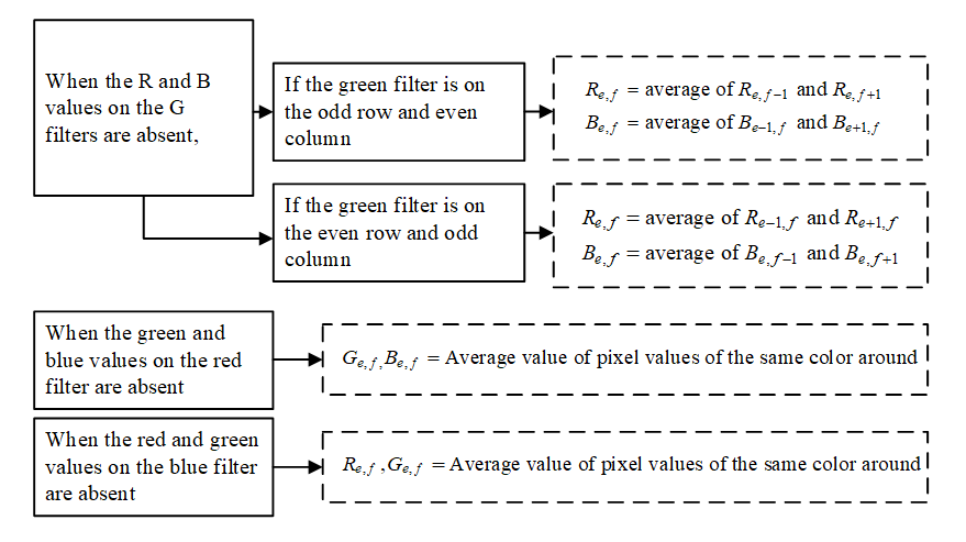
As shown in Fig.1, when the R and B values on the G filters are absent, the R and B values of the G filter are respectively calculated as follows if the green filter is on the odd row and even column:
|
Figure 2. Mechanism of bilinear interpolation algorithm. |
Compared with other algorithms, bilinear interpolation is the simplest linear algorithm. Calculation is straightforward but accuracy is compromised. Additionally, it cannot handle the zippering effect or the Moire fringe effect [6].
2.2. Cok algorithm
Cok algorithm is based on the optical mechanism. For the smooth neighbour areas of an object, there is no sharp edges on these areas and the ratio of each two colour channels has slight changes [7]. The algorithm steps are as follow.
Firstly, the green channel interpolation values can be computed with the bilinear algorithm. Secondly, use the ratio of contiguous red and blue pixel values to the green values to compute the red and blue color interpolation value. Suppose Rmn is the red channel interpolation value at mth row and nth column. Rij is the red pixel value at ith row and jth column. Gmn is the green pixel value at mth row and nth column. Gij is the green channel interpolation value at ith row and jth column. Bmn is the blue channel interpolation value at mth row and nth column. Bij is the blue pixel value at ith row and jth column. We can get the calculation method of Rmn and Rij as follows:
Rmn=GmnRijGijBmn=GmnBijGij
For multi-contiguous points, it is to compute the average of these ratios. An example is shown as follow. Suppose R66 is the red color interpolation value at sixth row and sixth column, and the position of other channels is expressed in the same way.
R66=G66R55G55+R57G57+R75G75+R77G774
Cok's approach has been shown to be successful, however it performs poorly at edges. In terms of colour transition, the Cok's algorithm is more sensible, but it is still unable to successfully maintain details. The linear transformation of pixel value will smooth images and make the edges and sharp corners unnatural [8].
2.3. Hibbard-Laroche algorithm
While Cok's technique is premised on the idea that the ratio of the luminance of these three colours is likely to be a constant, the Hibbard-Laroche algorithm uses the difference in luminance of RGB colours as a constant [9]. Gm,n represents a green channel of pixels at ith row and jth column. There are two important variables representing horizontal gradient α and vertical gradient β , If α \lt β , it indicates that there is a greater likelihood of edges in the vertical direction, in which case the interpolation of the green channel is the average of the values of the two green channels in the horizontal direction. Otherwise, the interpolation of the green channel is the average of the values of the two green channels in the vertical direction. Once all pixels’ green channel values are calculated, red and blue channel values can be computed. In terms of Laroche’s algorithm, what is different from Hibbard algorithm is that it uses a different method to set the vertical gradient and horizontal gradient:
\begin{matrix}α=|2*{R_{m,n}}-{R_{m,n-2}}-{R_{m,n+2}}| \\ β=|2*{R_{m,n}}-{R_{m-2,n}}-{R_{m+2,n}}| \\ \end{matrix}
To summarize the algorithms mentioned above, the easiest way of image optimization mainly lies in performing a bilinear interpolation of the known neighbouring pixels, which also leads to serious zipper effects [10]. Hibbard-Laroche algorithm is better than earlier algorithms in terms of avoiding mathematical issues and dramatic changes in colour. The colour transition becomes smoother, and the Moire effect is somewhat improved by the Hibbard-Laroche algorithm.
3. Methodology
3.1. Image interpolation with clustering approach
In this part, we use the clustering idea for the green and blue colour interpolation at red pixel. The main approach is to use the surrounding pixel colour to perform clustering and then compute the colour interpolation.
|
Figure 3. Schematic diagram of multi-channel imaging. |
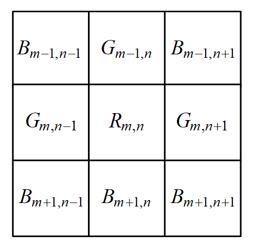
It is assumed that {R_{m,n}} , {G_{m,n}} , and {B_{m,n}} represent the pixel values of RGB at the positions of the m th row and the n th column, respectively. Then, for green colour interpolation, we use the difference of each two surrounding pixel to compute the colour distance: |{G_{m-1,n}}-{G_{m,n-1}}| , |{G_{m-1,n}}-{G_{m,n+1}}| , |{G_{m-1,n}}-{G_{m+1,n}}| , |{G_{m,n+1}}-{G_{m,n-1}}| , |{G_{m+1,n}}-{G_{m,n-1}}| and |{G_{m,n+1}}-{G_{m+1,n}}| . For the smallest distance, the corresponding green pixel will be classified into one cluster. Assuming the two pixel is {G_{m-1,n}} and {G_{m,n+1}} , then compute the average of these two pixels: {G_{v}}=({G_{m-1,n}}-{G_{m,n+1}})/2 . Then compute the remaining color distance: |{G_{m+1,n}}-{G_{m,n-1}}| , |{G_{m,n-1}}-{G_{v}}| , |{G_{m+1,n}}-{G_{v}}| . If the smallest distance among these three is |{G_{m+1,n}}-{G_{m,n-1}}| , then the green color interpolation at m th row and n th column will be {G_{v}} . Assuming the smallest distance among these three is |{G_{m,n-1}}-{G_{v}}| , then we need to judge whether {G_{m,n-1}} belongs to the {G_{m-1,n}} and {G_{m,n+1}} cluster. We use the Gaussian distribution for the judgement which is to compute the average μ and variance σ of these three pixel and if {G_{m,n-1}} \lt μ-2σ or {G_{m,n-1}} \gt μ+2σ , then {G_{m,n-1}} does not belong to this cluster. Otherwise, it belongs to the cluster. If {G_{m,n-1}} does not belong to the cluster, then {G_{v}} will be the green colour interpolation value of this pixel. Otherwise, {G_{m,n-1}} will be classified to the cluster. If {G_{m,n-1}} is classified to the cluster, we also use Gaussian distribution to judge whether {G_{m+1,n}} belongs to the cluster. If it does belong to the cluster, then the green color interpolation {G_{m,n}} will be the average of all four green pixels. Otherwise, the green colour interpolation {G_{m,n}} will be the average of the cluster. Moreover, if the green color interpolation {G_{m,n}} is the average of three pixels, For example, {G_{m,n-1}} , {G_{m-1,n}} , {G_{m,n+1}} . Then the blue color interpolation {B_{m,n}} will be the average of the two blue pixel which is contiguous to two of these three green pixels. In this example, it is {B_{m,n}}=({B_{m-1,n-1}}+{B_{m-1,n+1}})/2 . And the blue color interpolation will not process the clustering algorithm. Similarly, use the clustering idea to obtain the blue colour interpolation at red pixel. Then for red and green colour interpolation at blue pixel, use the same approach to get result.
As we obtain the colour interpolation at blue and red pixels, we can use the clustering idea to obtain the blue and red colour interpolation at green pixels or the red and green interpolation of blue pixels. Then we can use the clustering method at part 3.1 to obtain the multi-channel color interpolation value at the position of point.
3.2. Hibbard-based edge improvement algorithm
After the implementation of color interpolation based on clustering algorithm, this paper optimizes Hibbard algorithm to achieve de-mosaic of feature edges. This paper sets six variables and calculates the optimal parameters to calculate the green channel value for each pixel. Every variable is a gradient with a unique direction. The absolute different value between the real green channel value of the upper pixel and that of the lower pixel (Eq. 4) and the absolute different value between the real green channel value of the left pixel and that of the right pixel (Eq. 4) are used to represent vertical and horizontal gradients, respectively.
\begin{matrix}a=|{G_{m,n-1}}-{G_{m,n+1}}| \\ b=|{G_{m-1,n}}-{G_{m+1,n}}| \\ \end{matrix}
These values correspond to the variables set in the Hibbard algorithm. Additionally, diagonal gradients are taken into account. The diagonal gradients, which have an inclination to the left, are the absolute different value between the real green channel value of the left pixel and that of the lower pixel ( {c_{1}} from Eq. 5), and the absolute difference value between the real green channel value of the upper pixel and that of the right pixel ( {c_{2}} from Eq. 5). Diagonal gradient inclined to the left is expressed as:
\begin{matrix}{c_{1}}=|{G_{m,n-1}}-{G_{m+1,n}}| \\ {c_{2}}=|{G_{m-1,n}}-{G_{m,n+1}}| \\ \end{matrix}
The absolute values of the differences between the real green channel values of the left pixel and the upper pixel ( {d_{1}} from Eq. 6) and the real G channel values of the lower pixel and the right pixel ( {d_{2}} from Eq. 6) are diagonal gradients inclined to the right. Diagonal gradient inclined to the right is expressed as:
\begin{matrix}{d_{1}}=|{G_{m,n-1}}-{G_{m-1,n}}| \\ {d_{2}}=|{G_{m+1,n}}-{G_{m,n+1}}| \\ \end{matrix}
Threshold settings were established to increase accuracy, and only when the difference between diagonal gradients and vertical or horizontal gradients surpasses would the green channel value be computed using diagonal gradients.
The methods presented in this section approach extends the green channel values of all pixels by taking into account diagonal gradients, unlike the Hibbard algorithm, which only takes into account vertical and horizontal gradients. Meanwhile, the blue and red channel values are computed using the Hibbard algorithm. If the real green channel values of the pixel's four basic directions are identical, the pixel's remaining green channel value will be determined by the same value. The following is the pixel value calculation formula for the green channel value when an image's top, lower, left, and right pixels all have the same real green channel values:
{G_{m,n}}={G_{m,n-1}}
This section mainly considers the diagonal gradient under the green channel to complete the green channel interpolation. If {c_{1}} \lt {c_{2}} and {c_{1}} \lt 15 , the green channel value is computed by the average value of the real green channel pixel value on the left and that of the pixel at the bottom. The calculation equation is as follows:
{G_{m,n-1}}=\frac{{G_{m,n-1}}+{G_{m+1.n}}}{2}
However, if {c_{1}} \gt 15 ,which means the pixel lattice is likely to be on the boundary where the colour changes significantly. the variance of {G_{m,n-1}} , {G_{m,n+1}}{G_{m+1,n}} , {G_{m+1,n-2}} and {G_{m+2,n-1}} (the colour block at the bottom left of this pixel) is compared with the variance of {G_{m-1,n}} , {G_{m,n+1}} , {G_{m-2,n+1}} and {G_{m-1,n+2}} (the colour block on the top right of this pixel) to determine which colour block this pixel belongs to. It is assumed that the pixel belongs to the colour block at the bottom left of it (the variance is smaller), the G value of this pixel is equal to the average value of the real G value of the pixel on its left and that of the pixel at its bottom. Specially, if these two variances are equal, this pixel’s real red or blue channel value will be used for reference. For example, if this pixel has a real red channel value, it will compare with {R_{m+2,n-2}} and {R_{m-2,n+2}} to determine which colour block it belongs to. When the vertical or horizontal gradients are smaller, the pixel’s green channel value is calculated using Hibbard algorithm.
4. Experiment and analysis
4.1. Multi-channel color graphic interpolation using clustering approach
In this part, clustering approach is used to compare the zipper effect with bilinear algorithm, Cok algorithm and Hibbard algorithm at edge. Experiment result is shown as follow.
|
|
|
|
a) Clustering algorithm | b) Cok algorithm | c) Bilinear algorithm | d) Hibbard algorithm |
Figure 4. zipper effect comparative experiment. | |||


It is obvious that this algorithm eliminates the zipper effect at the edge. The performance is better than the other three algorithms. Then the comparison of diagonal edges both in artificial triangle and real pictures is shown below.
|
|
|
|
a) Clustering algorithm | b) Cok algorithm | c) Bilinear algorithm | d) Hibbard algorithm |
|
|
|
|
e) Clustering algorithm | f) Cok algorithm | g) Bilinear algorithm | h) Hibbard algorithm |
Figure 5. Optimization effect of image edge features. | |||

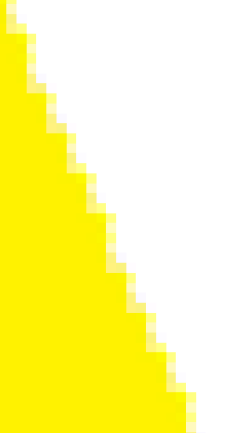
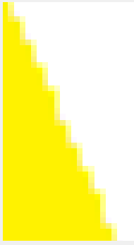
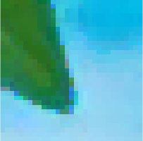


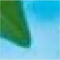
It is overt that the clustering algorithm can get sharper edges, and less blurry. Consequently, clustering algorithm can reach better result.
4.2. Image optimization based on improved Hibbard algorithm
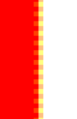
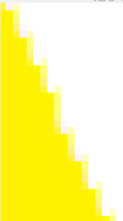
At present, edge extraction technology is an important cornerstone of target detection and matching technology. However, the edge feature of some images is vague due to the blurring of the edge feature, which makes it difficult to extract the edge. Therefore, after completing the experiment of color interpolation based on clustering algorithm, this paper conducts edge de-mosaic experiment for some images with blurred edges, and the results are as follows.
|
|
a) Result of Hibbard algorithm | b) Proposed algorithm |
Figure 6. Edge optimization of vector graphics. | |
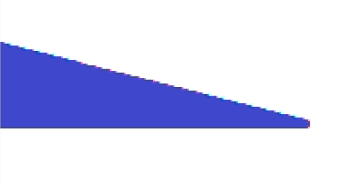
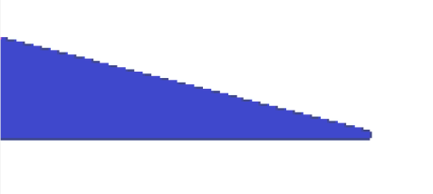
Through the comparison, it is obvious that the Fig. 6.(b) has more obvious edge gradient features in the oblique direction, thus facilitating edge feature extraction. The above experiments show that the algorithm proposed in this section performs well in vector graphics. It effectively eliminates the mosaic on the edge.
5. Conclusion
This paper first analyzes the significance of image interpolation in machine vision, and analyzes the three most common interpolation algorithms. Secondly, this paper introduces the idea of clustering into the image interpolation algorithm, and calculates the color interpolation by clustering the pixels around the multi-channel pixels in the image. Then, based on the traditional Hibbard algorithm, this paper considers the diagonal gradient around the pixel, and proposes a new improvement strategy. Finally, the analysis of the experimental results of several verifies that the algorithm proposed in this paper produces better results in the edge interpolation effect, and can better eliminate the zipper effect of the edge and obtain clearer edge features.
References
[1]. Tanaka M, Azuma H, Uchino S, et al 2012 Display device, US08203261B2[P].
[2]. Ogawa T and Adachi S 2014 Erratum to: Measurement of Moisture Profiles in Pasta During Rehydration Based on Image Processing[J]. Food & Bioprocess Technology 7(12):3655-3657.
[3]. John D M, Thomas A. Combined denoising and demosaicing of CFA images[C]// 2015 IEEE International Conference on Signal Processing, Informatics, Communication and Energy Systems (SPICES). IEEE
[4]. Bailey K. 2004. A novel approach to real-time bilinear interpolation[M]. IEEE Computer Society.
[5]. Chen L and Gao C M. 2007 Fast discrete bilinear interpolation algorithm[J]. Computer Engineering and Design.
[6]. Shi J, Kang C, S Xiong, et al. 2011 Edge-based image interpolation approach for video sensor network. IEEE.
[7]. Lu J. 2021 Analysis and Comparison of Three Classical Color Image Interpolation Algorithms[J]. Journal of Physics: Conference Series 1802(3):032124 (8pp).
[8]. Kimmel R. 1999 Demosaicing: image reconstruction from color CCD samples[J]. Image Processing IEEE Transactions on 8(9):1221-1228.
[9]. Laroche C A. 1994 Apparatus and method for adaptively interpolating a full color image utilizing chrominance gradients: US, US5373322 A[P].
[10]. Laroche C A, 1993 Prescott M A. Apparatus and method for adaptively interpolating a full color image utilizing chrominance gradients.
Cite this article
Hou,J.;Wang,Z.;Xie,Y.;Zhou,F. (2023). Research on RGB image optimization technology based on cluster analysis and improved Hibbard algorithm. Applied and Computational Engineering,4,119-126.
Data availability
The datasets used and/or analyzed during the current study will be available from the authors upon reasonable request.
Disclaimer/Publisher's Note
The statements, opinions and data contained in all publications are solely those of the individual author(s) and contributor(s) and not of EWA Publishing and/or the editor(s). EWA Publishing and/or the editor(s) disclaim responsibility for any injury to people or property resulting from any ideas, methods, instructions or products referred to in the content.
About volume
Volume title: Proceedings of the 3rd International Conference on Signal Processing and Machine Learning
© 2024 by the author(s). Licensee EWA Publishing, Oxford, UK. This article is an open access article distributed under the terms and
conditions of the Creative Commons Attribution (CC BY) license. Authors who
publish this series agree to the following terms:
1. Authors retain copyright and grant the series right of first publication with the work simultaneously licensed under a Creative Commons
Attribution License that allows others to share the work with an acknowledgment of the work's authorship and initial publication in this
series.
2. Authors are able to enter into separate, additional contractual arrangements for the non-exclusive distribution of the series's published
version of the work (e.g., post it to an institutional repository or publish it in a book), with an acknowledgment of its initial
publication in this series.
3. Authors are permitted and encouraged to post their work online (e.g., in institutional repositories or on their website) prior to and
during the submission process, as it can lead to productive exchanges, as well as earlier and greater citation of published work (See
Open access policy for details).
References
[1]. Tanaka M, Azuma H, Uchino S, et al 2012 Display device, US08203261B2[P].
[2]. Ogawa T and Adachi S 2014 Erratum to: Measurement of Moisture Profiles in Pasta During Rehydration Based on Image Processing[J]. Food & Bioprocess Technology 7(12):3655-3657.
[3]. John D M, Thomas A. Combined denoising and demosaicing of CFA images[C]// 2015 IEEE International Conference on Signal Processing, Informatics, Communication and Energy Systems (SPICES). IEEE
[4]. Bailey K. 2004. A novel approach to real-time bilinear interpolation[M]. IEEE Computer Society.
[5]. Chen L and Gao C M. 2007 Fast discrete bilinear interpolation algorithm[J]. Computer Engineering and Design.
[6]. Shi J, Kang C, S Xiong, et al. 2011 Edge-based image interpolation approach for video sensor network. IEEE.
[7]. Lu J. 2021 Analysis and Comparison of Three Classical Color Image Interpolation Algorithms[J]. Journal of Physics: Conference Series 1802(3):032124 (8pp).
[8]. Kimmel R. 1999 Demosaicing: image reconstruction from color CCD samples[J]. Image Processing IEEE Transactions on 8(9):1221-1228.
[9]. Laroche C A. 1994 Apparatus and method for adaptively interpolating a full color image utilizing chrominance gradients: US, US5373322 A[P].
[10]. Laroche C A, 1993 Prescott M A. Apparatus and method for adaptively interpolating a full color image utilizing chrominance gradients.