1. Introduction

Nowadays, Fundamental Analysis and Technical Analysis have long been used by investors as an analysis instrument to predict the stock price in gaining optimal return [1]. However, this combination is not mentioned widely in Chinese stock market. In this work, we use technical momentum (Time-Series and Cross Sectional) to predict future trends based on a security performance over a certain period of time and compared with the performance of other securities in the market. Meanwhile, fundamental factors including Return on Equity(ROE) and a combination of Profitability, Debt Management, Assets Management(PDA) help to make an in-depth analysis of the company's financial situation and assess its liquidity, debt management and asset management. Hence, this strategy can enhance investors' ability to control investment risks and adapt to market dynamics.

2. Data

2.1. Data Universe

The universe of our strategy includes the stocks in CSI 300. On the one hand, the CSI 300 index is the first cross-market index legally authorized by the Shanghai and Shenzhen exchanges and consists of the most representative 300 securities, most of which are from traditional industries, cyclical industries and mature industries, and their business development has entered a mature stage with relatively stable performance. Meanwhile, our universe is dynamic because the securities in CSI 300 change nearly every 6 months according to the performance of the securities. Therefore, to diminish the survivor-ship bias and keep the number of the stocks in our universe almost the same in every year, we constantly adjust our universe according to the real situations of CSI 300 and the frequency is every 6 months.

2.2. Data Sets

The following Data Sets are necessarily utilized to calculate our alphas:

Data Set 1: (Stocks' Daily Trading Information)

StockCode, Date(daily), Close Price, Open Price, High Price, Volumn, Market Value

Data Set 2: (Balance Sheet)

StockCode, Date(quarterly), Total Asset, Current Asset, Total Debt, Current Liabilities, Total

Common Equity, Inventory, Account Receivable

Data Set 3: (Income Statement)

StockCode, Date(quarterly), Net Income, Sales, Interest Expense, IncomeTaxExpense

2.3. Data Sources

The main data used in this study is from CSMAR, which is the largest and most accurate financial and economic database in China. CSMAR covers China's securities, futures, foreign exchange, macro, industry and other major economic and financial fields of high precision research database. It is widely used as a basic tool for investment and empirical research.

2.4. Date Range

In-sample Date: 2014.01.01-2021.12.31 (8 years)

Out-of-Sample Date: 2022.01.01-2024.03.31 (2 years and 1 quarter)

We divide the ten years to 8 years and 2 years and a quarter because eight years can help us to test our strategies with more data and 2019-2021 are Covid period, which can give us special values to make analysis.

3. Alphas

3.1. PDA-T (PDA with Time-series and Cross-Sectional Momentum)

3.1.1. Economic Intuition

In this alpha, we explore two factors, TCM (Time-Series Momentum and Cross-Sectional Momentum) and PDA (Profitability-Debt-Asset) to capture different types of market signals and optimize portfolio performance. To elaborate further, in PDA, we analyze the fundamental statements by calculating Current Ratio, Debt Ratio, DSO and combining with EBIT so that we can get the ranks of Liquidity, Debt Management and Asset Management of companies. At the same time, we utilize TCM to perform both horizontal and vertical analyses of issued stocks. After the combination of TCM and PDA with dot product, the results of our Alpha can find out it reasonable to long the stocks with good performance and rising trend, and short the stocks with poor performance and declining trend.

3.1.2. PDA-T

Time-Series Momentum is based on the idea that an asset's past performance trend will continue into the future. Investors typically review an asset's price performance over a specific period, like the last 12 months, to forecast its future price trend [2]. Additionally, Cross-Sectional Momentum involves comparing the performance of various assets at a single point in time. This approach involves ranking assets based on the ratio of today's price to the price over a past period, such as six months, and then buying the assets with high rank and selling those with low rank [3]. Meanwhile, Profitability-Debt-Asset Analysis offers a traditional and detailed method to evaluate a company's profitability, short-term and long-term solvency and capital turnover efficiency [4].

In practice, this strategy first screens out strong or weak stocks in the market through temporal momentum and cross-sectional momentum. These stocks are then subjected to in-depth fundamental analysis to assess their financial health, profitability, growth potential and market positioning to ensure that each investment decision is backed by solid value.

3.1.3. Alpha Formula

\( \begin{cases} \begin{array}{c} \begin{array}{c} PDA(Profitability-Debt-Asset)=\frac{EBIT}{MarketValue}×[rank(CR)+rank(\frac{1}{DR})+rank(\frac{1}{DSO})] \\ TCM(Time SeriesCross Sectional)=[\frac{close price(today)}{12-month moving average of close price}-1]× \\ rank(\frac{close price(today)}{close price(6-month ago)}) \\ PDA-T=exp(PDA)⊙TCM \end{array} \ \ \ (1) \\ \end{array} \end{cases} \)

Exp() ensures this index is positive and will not disrupt the rank sequence of PDA.

To satisfy the two constraints of Alpha Matrix, we demean and normalize all non-zero values.

Formula Sheet:

\( CR(Current Ratio)=\frac{Current Asset}{Current Liabilities}       \ \ \  （2） \)

\( DR(Debt Ratio)=\frac{Total Liabilities}{Total Asset}       \ \ \  （3） \)

\( DSO=\frac{Account Receivable}{\frac{Sales}{365}}       \ \ \  （4） \)

3.1.4. In-Sample PnL Result

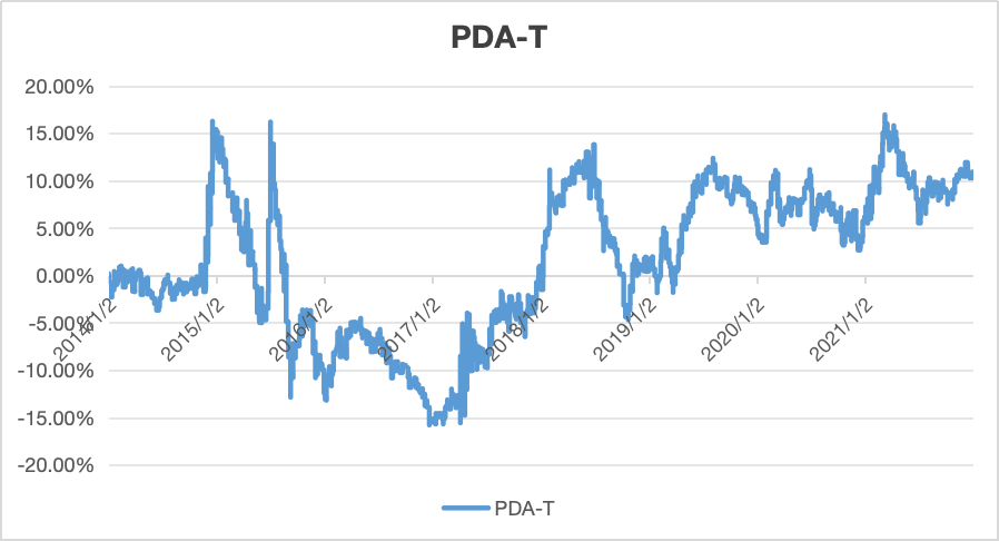
Figure 1: Cumulative PnL of PDA-T (Before execution costs) Changes with Time(GMV=100,000,000¥)

Fig.1 tracks a trading strategy from January 1, 2014, to December 31, 2021, reveals a trajectory marked by the strategy's performance through various economic phases. Initially, the trend shows low PnL up to 2016 and this bottom line possibly indicates a coming developmental phase. Meanwhile, Fig.1 shows that the PnL experienced heightened volatility between mid-2016 and 2018, likely exacerbated by global events like Brexit and shifts in U.S. monetary policy, which shows this strategy is a approach sensitive to international market dynamics [5,6]. This turbulent period might have tested and refined the strategy’s risk parameters, leading to a period of recovery and gradual gains that peaked around early 2020, demonstrating an improved risk-return profile and alignment with pre-pandemic market stability. The COVID-19 pandemic introduced extreme volatility, yet the strategy’s ability to quickly recover highlights its resilience and the necessity of dynamic risk management to handle rapid market changes effectively [7,8]. Overall, the strategy, while potentially profitable, underscores the need for sophisticated management to maintain a balance between risk and return, given its sensitivity to macroeconomic shifts and global market sentiments.

3.1.5. In-Sample Performance Statistics

Table 1: PDA-T In-Sample Performance

The annualized return is 1.365% , lower than the expected annualized return of 0.05~0.07. The annualized volatility is about 12.488% which is between the range of 0.1~0.2; thereby, it is acceptable. The information ratio is about 0.109 which is little higher than 0.1; thus, it is exceptional. The Sharpe Ratio is about -0.028 while the max drawdown is 32.048%. The information coefficient is 0.006, extremely close to zero, so it can be recognized as no apparent linear relation.

3.2. ROE-T (ROE with Time-series and Cross-Sectional Momentum)

3.2.1. Economic Intuition

In this alpha, we explore two factors, ROE and TCM and we use DuPont Analysis to dissect ROE. Be detailed, DuPont Analysis, a typical method to evaluate the profitability of companies, decomposes ROE to Profit-Margin, Total-Asset-Turnover and Equity-Multiplier, which is helpful to make deep analyses and comparisons of business performance [9]. Meanwhile, we use TCM to analyze issue stocks horizontally and vertically. In the same manner, our alpha is the combination of TCM and ROE with dot product, whose results show that it is reasonable to long the stocks with good performance and rising trend, and short the stocks with poor performance and declining trend in this method.

3.2.2. ROE-T

Different from PDA-T, ROE-T can better reflect a company's ability to return on investment. TCM is the same as we mentioned before in the PDA-T.

The investment portfolio leverages ROE and TCM metrics to identify stocks with high profitability and promising momentum trends, aiming to maximize returns and minimize risks. ROE-T combines traditional ROE analysis with Time-Series and Cross-Sectional Momentum, allowing us to pinpoint companies that not only have strong profitability but also show stable growth prospects. Concurrently, TCM helps identify stocks with superior historical performance and those outperforming peers, ensuring our selections have both past success and ongoing momentum. Our portfolio construction focuses on diversification across sectors and regular re-balance based on up-to-date metrics, aimed at achieving higher-than-average market returns while maintaining risk at a managed level.

3.2.3. Alpha Formula

\( \begin{cases} \begin{array}{c} \begin{array}{c} ROE=(ProfitMargin×TotalAssetTurnover)×EquityMultiplier \\ TCM(Time SeriesCross Sectional)=[\frac{close price(today)}{12-month moving average of close price}-1]× \\ rank(\frac{close price(today)}{close price(6-month ago)}) \\ ROE-T=exp(ROE)⊙TCM \end{array} \ \ \ (5) \\ \end{array} \end{cases} \)

Exp() ensures this index is positive and will not disrupt the rank sequence of ROE.

To satisfy the two constraints of Alpha Matrix, we demean and normalize all non-zero values.

Formula Sheet:

\( Profit Margin=\frac{Net Income}{Sales}       \ \ \  （6） \)

\( Total Asset Turnover=\frac{Sales}{Total Asset}       \ \ \  （7） \)

\( Equity Multiplier=\frac{Total Asset}{Equity}       \ \ \  (8) \)

3.2.4. In-Sample PnL Results

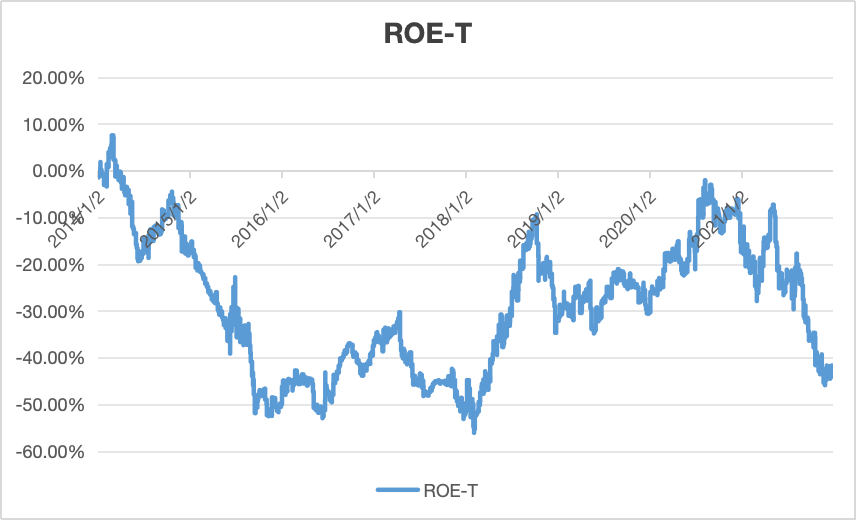
Figure 2: Cumulative PnL of ROE-T (Before execution costs) Changes with Time (GMV=100,000,000¥)

Between 2014 and 2021, the cumulative PnL of stocks chosen by ROE-T experienced significant fluctuations influenced by various economic and political factors. From February 2014 to December 2015, the cumulative PnL plummeted from 10% to negative 50% due to the Fed raising interest rates multiple times, leading to capital outflows from the Chinese market and devaluation of the Chinese currency. This had a negative impact on the Chinese economy and many enterprises' capital management, exacerbated by the dramatic Chinese stock market crash in June 2015, whose effects lingered for several years. From 2016 to March 2017, the cumulative PnL slightly recovered to minus 30% as the pace of interest rate increases slowed and the government prioritized economic stabilization. However, from 2017 to February 2018, the cumulative PnL declined again to minus 55% due to US President Donald Trump's expansionary fiscal policy and the Fed's three interest rate hikes, negatively impacting the Chinese market [10]. A turnaround occurred between 2018 and October 2018, with the cumulative PnL rising to minus 10% amid the easing of Sino-US trade frictions, improved market risk appetite, increased investor confidence, relaxed financing channels, foreign capital inflows, and tax reduction policies optimizing liquidity structures and reducing financial burdens, thus enhancing corporate profitability. However, from 2019 to 2021, the cumulative PnL entered a small trough due to the adverse impacts of the COVID-19 pandemic on supply chains and capital flows, which deteriorated profitability and operational conditions for enterprises.

3.2.5. In-Sample Performance Statistics

Table 2: ROE-T In-Sample Performance

The annualized return is about -5.506% which is undesirable. The annualized volatility is about 18.806% and is acceptable. The information ratio is about -0.293 and the sharpe ratio is about -0.384, which are negative, so they are not satisfactory. The max drawdown is 63.613% and needs improvement. The information coefficient is -0.0169, fairly near to zero, so it can be supposed as no apparent linear relation.

4. Refinement

4.1. Sector Neutralization

4.1.1. Description

Sector Neutralization divides all stocks into 6 different sectors (Finance, Utilities, Properties, Conglomerates, Industrials, Commerce) and realize market neutralization in every sector. This approach reduces systemic risk, improves the precision of individual stock selection, and optimizes the risk distribution of the portfolio [11], so that the cumulative PnL shows a more stable and sustained growth over the whole time period.

4.1.2. PDA-T

\( Refined PDA-T =\frac{Raw PDA-T-mean(all PDA-T in sector)}{\sum |Raw PDA-T-mean(all PDA-T in sector)|}       \ \ \  (9) \)

In-sample PnL Results

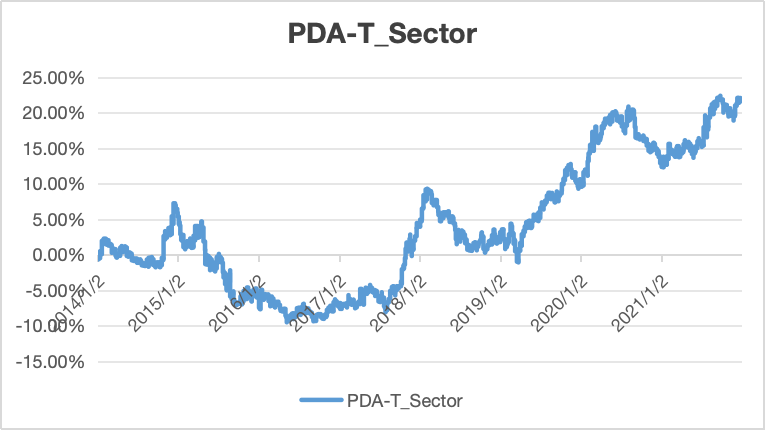
Figure 3: Cumulative PnL of PDA-T(Before execution costs) Changes with Time (After Sector Neutralization)(GMV=100,000,000 ¥)

By neutralizing the industry, the cumulative PnL volatility of PDA-T is significantly reduced and the performance is more stable. Specifically, from the beginning of 2014 to the beginning of 2015, the cumulative PnL of both Fig.1 and Fig.3 grew to 5%; From the beginning of 2015 to the beginning of 2016, the cumulative PnL of Fig.1 fell sharply by 20% to -15%, while Fig.3 only fell by 10% to -5%, with significantly less volatility. From 2016 to 2017, Fig.3 PnL fluctuated between -5% and -10%, which is smaller than the fluctuation in Fig.1. From 2017 to 2018, the cumulative PnL for Fig.1 fell by 15% to -20%, while Fig.3 fell by only 5% to -10%. From early 2018 to early 2019, Fig.3 PnL rebounded by 10% to 0, showing greater resilience. From 2019 to 2021, Fig.1 fluctuated greatly, while Fig.3 shows a continuous increase in cumulative PnL to 25%, showing greater investment stability and overall performance. In short, industry neutrality effectively improves the precision of individual stock selection and the risk diversification effect of investment portfolio.

Performance Statistics

Table 3: PDA-T In-Sample Performance After Sector-Neutralization

After refinement, all statistics have improvements. The annualized return is 2.750%, still lower than the expected annualized return of 0.05~0.07, but has a increase compared with previous 1.365%. The annualized volatility is about 6.380%, lower than previous 12.488%. The information ratio is about 0.431, higher than previous 0.109. The sharpe ratio is about 0.161, higher than previous -0.028. The max drawdown is 16.742%, lower than previous 32.048%. The information coefficient is 0.025, very near to zero, so it can be seen as no apparent linear relation.

4.1.3. ROE-T

\( Refined ROE-T =\frac{Raw ROE-T-mean(all ROE-T in sector)}{\sum |Raw ROE-T-mean(all ROE-T in sector)|}       \ \ \  (10) \)

In-sample PnL Results

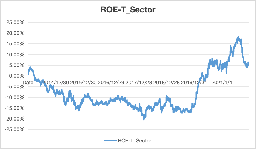
Figure 4: Cumulative PnL of ROE-T(Before execution costs) Changes with Time (After Sector Neutralization)(GMV=100,000,000 ¥)

Through sector neutralization, the performance of cumulative PnL become more stable and exceptional. Between 2015 and 2016, the drop off of cumulative PnL was much more alleviated; the bottom point was about minus 15% in December 2015 after refinement, 35% higher than before refinement. The lowest point was about minus 20% in February 2018 after refinement, 35% higher than the minimum value in January 2018 before refinement. Between 2020 and 2021, the surge of cumulative PnL was much more dramatic; it increased sharply from minus 15% to 15% after refinement, while the highest point was below zero point before refinement.

In Chinese stock market between 2014 to 2021, the transformation of economic structure made the proportion of service industry increase, while the investment in infrastructure and real estate decreases, which led to the fluctuation of stock performance in specific industries, while the sector neutralization strategy can effectively diversify investment risks and prevent stocks from relying on the fluctuation of specific industries. Additionally, the registration system reform promoted the rapid development of high-tech and innovative enterprises, and the sector neutralization strategy benefits from these emerging areas by better capturing the overall growth of the market by diversifying investment. Moreover, the sector neutralization can achieve the optimization of the market structure and the recovery of the supply chain after the COVID-19 pandemic by stabilizing the impact of business cycle fluctuations on specific industries.

Performance Statistics

Table 4: ROE-T In-Sample Performance After Sector-Neutralization

After refinement, all statistics have improvements. In particular, the annualized return, information ratio and sharpe ratio become positive figures. The annualized return is about 0.603%, increasing 12.109%. The information ratio is about 0.078 and the sharpe ratio is about -0.144, still a little low, so they are not satisfactory. The annualized volatility declines from 18.806% to 7.731% and is excellent. The max drawdown reduces from 63.613% to 24.502%, match the interval of 20%~25%; hence, it is perfect. The information coefficient is 0.005, meaning no apparent linear relation.

4.2. Ranking Filter

4.2.1. Description

In this refinement, we remove the exponent of PDA/ROE and replace it with Rank. It can get rid of the stocks which have high TCM but Low PDA/ROE or those have low TCM but High PDA/ROE. Because we could not explain why the fundamental factors and technical factors behave oppositely, we prefer to filter these parts and only use those stocks whose PDA/ROE and TCM behave in the same direction.

The ranking was carried out among all the 600+ stocks from 2014 to 2024Q1 (and then the overlapped parts with the actual 300 stocks were selected). However, we observed that among these 600+ stocks, the number of stocks with positive TCM was much smaller than that with negative TCM. Therefore, we will expand the range of stocks with high PDA/ROE ranking to more than 200(rather than half of the total number of stocks), so that the filtered stocks will not be too few and avoid excessive concentration of funds.

4.2.2. PDA-T

\( Refined PDA-T=\begin{cases} \begin{array}{c} \begin{array}{c} 0, if Rank(PDA)≥200 and TCM \lt 0 \\ 0, if Rank(PDA) \lt 200 and TCM≥0 \\ Rank(TCM), if Rank(PDA) \lt 200 and TCM \lt 0 \\ Rank(TCM), if Rank(PDA)≥200 and TCM≥0 \end{array} \\ \end{array} \end{cases}\ \ \ (11) \)

In-Sample PnL Result

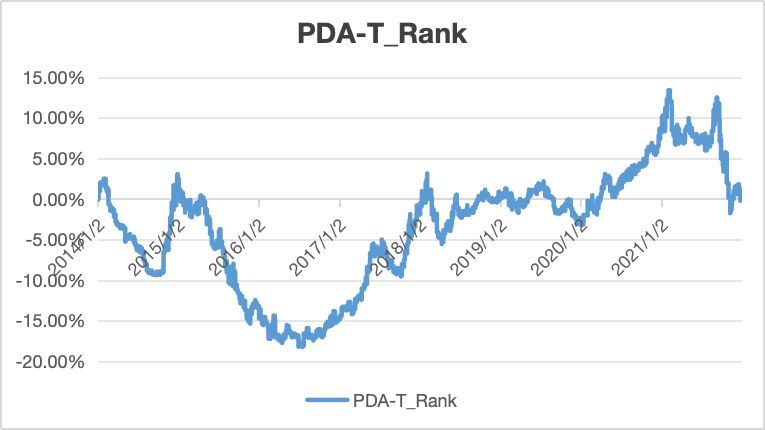
Figure 5: Cumulative PnL of PDA-T(Before execution costs) Changes with Time (After Ranking Filter)(GMV=100,000,000 ¥)

By applying the Ranking Filter strategy, the volatility of the cumulative PnL of PDA-T is significantly reduced, and the performance is more stable. Specifically, from the beginning of 2015 to the beginning of 2016, the cumulative PnL of the adjusted chart decreased by 15%, while the original chart decreased by 20%. From 2017 to 2018, the adjusted chart decreased by only 5%, while the original chart was 15%. From the beginning of 2018 to the beginning of 2019, the cumulative PnL of the adjusted chart rebounded from -15% to -5%, a rebound of 10 million. From 2019 to 2021, the adjusted chart showed a continuous upward trend, with the cumulative PnL increasing from -5% to 10%. This strategy filters out stocks with high TCM but low PDA or low TCM but high PDA. Therefore, this Ranking Filter strategy effectively reduces the impact of market fluctuations and improves the stability and the returns of the investment portfolio.

Performance Statistics

Table 5: PDA-T In-Sample Performance After Ranking-Filter

In this refinement, the annualized volatility and the maximum drawdown both decreased significantly, to 6.616% and 21.266% respectively. However, the annualized return yield is also down to 0.015%, and the Sharpe ratio and IR are all low, so this is not a very valuable refinement. The information coefficient is 0.00013, meaning no apparent linear relation.

4.2.3. ROE-T

\( Refined ROE-T=\begin{cases} \begin{array}{c} 0, if Rank(ROE)≥200 and TCM \lt 0 \\ 0, if Rank(ROE) \lt 200 and TCM≥0 \\ Rank(TCM), if Rank(ROE) \lt 200 and TCM \lt 0 \\ Rank(TCM), if Rank(ROE)≥200 and TCM≥0 \end{array} \end{cases}\ \ \ (12) \)

In-sample PnL Result

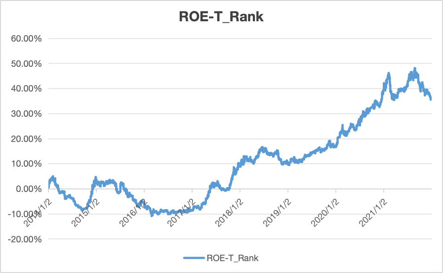
Figure 6: Cumulative PnL ROE-T(Before execution costs) Changes with Time (After Ranking Filter)(GMV=100,000,000 ¥)

Through ranking filter, the stability and profitability has a significant enhancement. The basin trough between 2015 and 2019 was less conspicuous after refinement; the bottom point was about minus 10% in 2016 after refinement, 40% lower than the data in 2016 before refinement. The growth started from the year of 2018 was more steady and the growth rate was more consistent after refinement than before. The cumulative PnL reached almost 50 million in 2021 after refinement, 50 million higher than the maximum level of the cumulative PnL in 2021 before refinement.

Performance Statistics

Table 6: ROE-T In-Sample Performance After Ranking-Filter

After refinement, all statistics have enhancement. In particular, the annualized return, information ratio, sharpe ratio and information coefficient become positive figures. The annualized return is about 0.603%, increasing 9.994%. The information ratio is about 0.603, in the range of 0.4~0.7, so it can be considered as good. The sharpe ratio is 0.372, even not quite high, but it is 0.756 higher than before. The annualized volatility declines 11.365% and the max drawdown reduces 47.805%; hence, they are perfect. The information coefficient is 0.035, regarding no apparent linear relation.

4.3. Combination

4.3.1. Description

At the very beginning, we combine the refined PDA-T (After Ranking Filter and Sector Neutralization) and refined ROE-T (After Ranking Filter and Sector Neutralization) with weight of 50:50. Then, the weights of PDA-T and ROE-T in combination are modified every year and the ratio equals to the ratio of the cumulative PnL of PDA-T and ROE-T from the previous year and we keep the absolute sum of weights equal to 1.

4.3.2. Execution Cost

We decide commission costs as 0.03% of the transaction value according to KPMG's Mainland China Securities Survey 2021.

4.3.3. Results

Figure 7: Cumulative PnL(Combination) Changes with Time(GMV=100,000,000 ¥)

Before Execution Cost:

After combining these two refinements, we get a new cumulative graph of PnL. As can be seen from Fig.7, the portfolio experiences a significant decline in profitability in mid 2015 and keeps the low position until mid 2016. Especially, in mid 2016, the decline was the most severe and the cumulative profit and loss once fell below -15%. After the lowest point of 2016, the trends starts increasing. However, it stops at the beginning of 2018 and the highest point of the PnL is lower than 15%. Meanwhile, since early 2018, the cumulative PnL shows a continuing slowdown and the rise is almost insignificant.

After Execution Cost:

The graph of the overall trend of PnL after execution cost is almost the same as the one before execution cost. However, as we can see in Fig.7, the PnL finally falls on the negative value (about -5%), which means this portfolio may not behave as well as we expect.

4.3.4. Performance Statistics

Table 7: Combination In-Sample Performance

Before Execution Cost:

The annualized return is 0.411%, which looks not that remarkable but still makes profits. The annualized volatility is 5.713%, which means the risk of the portfolio is acceptable. Meanwhile,information ratio is low and sharpe ratio is negative and it reflects that the portfolio is only slightly outperforming its benchmark after adjusting for risk but still underperforming when compared to a risk-free investment. The information coefficient is still low.

After Execution Cost:

After considering execution cost, the annualized return becomes negative at -0.574%, which means the cost are high enough to erase the profits of the combination portfolio. It is worthy to mention that the information ratio becomes negative and the max drawdown increases to 21.209%. After execution cost, the lowest point becomes worse and the portfolio's risk-adjusted performance is worse than the benchmark.

5. Out-of-Sample

5.1. Final Selection

Refined PDA-T After Sector Neutralization: As Fig.3 and Table.5 we show above, the annualized return of PDA-T after Sector Neutralization is 2.75%, which is almost the double of the original PDA-T and 183 times of the PDA-T after Ranking Filter.

Refined ROE-T After Ranking Filter:As Fig.6 and Table.8 we show above, the annualized return of ROE-T after Ranking Filter is 4.488%, which increases almost 10% from the original ROE-T and 4% from the ROE-T after Sector Neutralization.

5.2. Refined PDA-T After Sector Neutralization

5.2.1. Out-of-Sample PnL Results

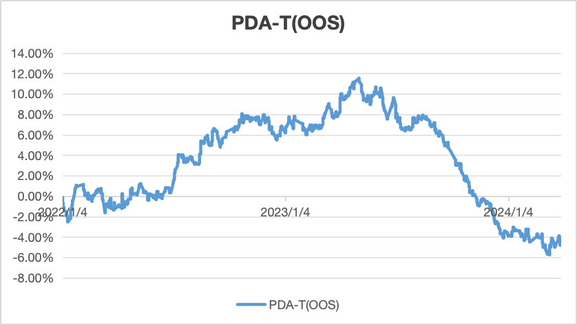
Figure 8: Cumulative PnL of PDA-T(OOS) Changes with Time(GMV=100,000,000 ¥)

In the out-of-sample data, the cumulative profit and loss curve of the PDA-T strategy showed steady growth from early 2022 to mid-2023, reaching a stage peak. However, it then began to fluctuate significantly and experienced a continuous downward trend from the end of 2023 to the beginning of 2024. This shows that the strategy encountered challenges in responding to market changes. Although there were certain signs of stability in early 2024, the overall curve still showed the need to re-evaluate and optimize the strategy to adapt to the current market dynamics.

5.2.2. Performance Statistics

Table 8: PDA-T Out-of-Sample Performance

Compared with the In-Sample data, although the annualized volatility and maximum drawdown have decreased, the annualized return has changed from 2.75% to -1.601% while the information ratio and sharpe ratio are negative, which means the behavior of the portfolio is still worse than the benchmark. Overall, although the strategy differs from the expected results, the deviation is not large, and the strategy parameters need to be re-estimated and adjusted to adapt to the latest market environment.

5.3. Refined ROE-T After Ranking Filter

5.3.1. Out-of-Sample PnL Results

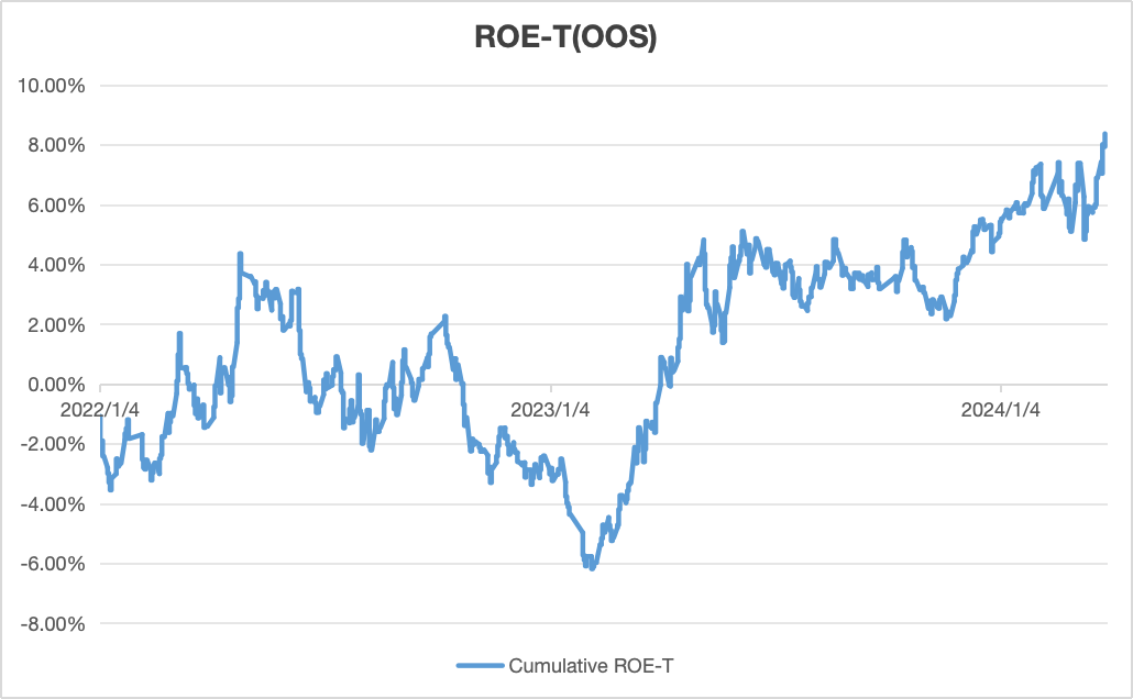
Figure 9: Cumulative PnL of ROE-T(OOS) Changes with Time(GMV=100,000,000 ¥)

In the out-of-sample data, the cumulative PnL of ROE-T fluctuated and showed a uptrend. In the first quarter of 2022, it increased to 4 million. Then, it declined to minus 6 million in the beginning of 2023. After that, it increased 11 million to 5 million in the first quarter of 2023, and remained in the approximate level. The out-of-sample data makes an acceptable performance, since it shows that the portfolio earned about 8 million at the end.

5.3.2. Performance Statistics

Table 9: ROE-T Out-of-Sample Performance

Compared with the in-sample data, its annualized volatility is worse while the annualized volatility keeps the same. Its information ratio and sharpe ratio are smaller, which means the portfolio construction is risky and may suggest greater volatility and a higher tracking error. However, the max drawdown works better from 15.808% to 10.537%. The information ratio is approximately near to zero, which means no apparent linear relation.

5.4. Combination (Out-of-Sample)

5.4.1. Out-of-Sample PnL Results

Figure 10: Cumulative PnL(Combination-OOS) Changes with Time(GMV=100,000,000 ¥)

Before Execution Cost:

In the out-of-sample data before adding execution costs, the cumulative PnL of combining two alphas results in a negative performance. In 2022~2023, the accumulative PnL presents an increasing trend and reaches a peak of 4 million in September 2023. However, this tendency does not last for the following time period. In 2023~2024, it declines rapidly to a minimum point to about 10 million in the end of 2023.

After Execution Cost:

After adding execution costs, the total trend of the cumulative PnL of combining two alphas is similar with the previous one. It shows a negative profitability as a whole, and is slightly lower than the former. Furthermore, the difference in cumulative PnL is small at first but grows larger and larger as time passed. Its final value is about 2 million in the end of 2023.

5.4.2. Performance Statistics

Table 10: Combination Out-of-Sample Performance

Before Execution Cost:

Generally, the cumulative PnL of combining two alphas before adding execution costs shows an adverse result in annualized return, IR and sharpe ratio; these figures are all below zero, demonstrating it has a profit liability. Admittedly, the annualized volatility and max drawdown are perfect; still, they cannot compensate for the loss of this portfolio. Besides, IC shows it has no apparent linear relation.

After Execution Cost:

After adding execution costs, the total statistics of the cumulative PnL of combining two alphas is similar with the previous one. Its annualized return, IR, sharpe ratio and max drawdown are a little bit worse than the former.

5.5. Trading Recommendation

5.5.1. PDA-T

On account of our overall analysis of the strategies, we do not recommend the refined PDA-T after sector neutralization as an alpha. Although it makes an all-around enhancement of all statistics compared with raw alpha with in-sample data, it does not maintain a good performance with out-of-sample data. With the overall trend is first up and then down, its annualized return is -1.601%, meaning the strategy will lose money on the whole. The probable reason is that the market fluctuation or emergency happened between 2023 and 2024 struck the strategy. Therefore, we do not recommend to use it directly but make further improvement.

5.5.2. ROE-T

According to our integrated analysis of the strategies, we recommend the refined ROE-T after ranking filter as an alpha. After refinement, the ROE-T strategy turns to make profits with in-sample data; its annualized return is 4.488%, 9.994% higher than before. In addition, its annualized volatility, IR, sharpe ratio and max drawdown are beyond our expected values with out-of-sample data. Therefore, we highly recommend the ROE-T after ranking filter due to its extraordinary performance with both in-sample and out-of-sample data.

5.5.3. Combination

Based on our comprehensive analysis and refined strategies, we do not recommend the combination of the refined PDA-T strategy after sector neutralization and the refined ROE-T strategy after ranking filter for trading within the CSI 300 universe. The annualized return and information ratio of out-of-sample data drops dramatically to negative.

6. Conclusion

In this paper, the hybrid strategy uses fundamental and technical analysis to design a profitable portfolio with data from CSI 300 to understand rapid growth and diversification of Chinese market. Two alpha models are used in the strategy: PDA-T and ROE-T. The two models assure that the portfolio is backed by solid economic intuition through selecting stocks based on history performance of a certain stock and performance of different stocks over the same period and by assessing companies’ financial health, profitability, growth potential and market positioning. Meanwhile, the research includes two refinement of strategies, which are industry neutralization and ranking filter, to improve stability and return of strategies. In the end, the recommended strategy is ROE-T after ranking filter because it performs well with both in-sample and out-of-sample data. Nevertheless, there is some room for improvement, such as increasing the annualized return of this strategy by using leverage and optimizing capital allocation, and augmenting sharpe ratio by controlling risks and enlarging sample universe.

References

[1]. Agustin, Isnaini Nuzula. “The Integration of Fundamental and Technical Analysis in Predicting the Stock Price.” Jurnal Manajemen Maranatha 18, no. 2 (May 27, 2019): 93–102. https://doi.org/10.28932/jmm.v18i2.1611.
[2]. Tobias J. Moskowitz , Yao Hua Ooi, Lasse Heje Pedersen, and Abstract We document significant “time series momentum” in equity index. “Time Series Momentum.” Journal of Financial Economics, December 11, 2011. https://www.sciencedirect.com/science/article/pii/S0304405X11002613.
[3]. Jegadeesh, Narasimhan, and Sheridan Titman. “Cross-Sectional and Time-Series Determinants of Momentum Returns.” Review of Financial Studies 15, no. 1 (January 2002): 143–57. https://doi.org/10.1093/rfs/15.1.143.
[4]. Abarbanell, Jeffrey S., and Brian J. Bushee. “Fundamental Analysis, Future Earnings, and Stock Prices.” Journal of Accounting Research 35, no. 1(1997):https://doi.org/10.2307/2491464.
[5]. AZIZ, Tariq, Jahanzeb MARWAT, Sheraz MUSTAFA, and Vikesh KUMAR. “Impact of Economic Policy Uncertainty and Macroeconomic Factors on Stock Market Volatility: Evidence from Islamic Indices.” The Journal of Asian Finance, Economics and Business 7, no. 12 (December 31, 2020): 683–92. https://doi.org/10.13106/jafeb.2020.vol7.no12.683.
[6]. Li, Ziyuan. “The Impact of the Federal Reserve’s Interest Rate Hike on the Chinese Economy.” Highlights in Business, Economics and Management 20 (November 30, 2023): 95–98. https://doi.org/10.54097/hbem.v20i.12325.
[7]. Evenett, Simon J. “Chinese Whispers: Covid-19, Global Supply Chains in Essential Goods, and Public Policy.” Journal of International Business Policy 3, no. 4 (November 4, 2020): 408–29. https://doi.org/10.1057/s42214-020-00075-5.
[8]. Xu, Zhitao, Adel Elomri, Laoucine Kerbache, and Abdelfatteh El Omri. “Impacts of Covid-19 on Global Supply Chains: Facts and Perspectives.” IEEE Engineering Management Review48,no.3(September1,2020):153–66. https://doi.org/10.1109/emr.2020.3018420.
[9]. Soliman, Mark T. “The Use of Dupont Analysis by Market Participants.” The Accounting Review 83, no. 3 (May 1, 2008): 823–53. https://doi.org/10.2308/accr.2008.83.3.823.
[10]. Chen Guo, and Zhang Xue Jiao. "Depth Review Series: The U.S. Interest Rate Hiking Cycle from 2015 to 2018." Investment Strategy Theme Report, Essence Securities Co., Ltd., August2, 2021. https://www.fxbaogao.com/detail/2777151
[11]. Ehsani, Sina, Campbell R. Harvey, and Feifei Li. "Is Sector-Neutrality in Factor Investing a Mistake?" SSRN, February 22, 2022. https://ssrn.com/abstract=3959116
Cite this article
Wang,R.;Zhu,J.;Han,Q.;Zhang,Y. (2025). A Hybrid Strategy Combined Multiple Fundamental and Technical Factors in CSI 300. Applied and Computational Engineering,134,24-40.
Data availability
The datasets used and/or analyzed during the current study will be available from the authors upon reasonable request.
Disclaimer/Publisher's Note
The statements, opinions and data contained in all publications are solely those of the individual author(s) and contributor(s) and not of EWA Publishing and/or the editor(s). EWA Publishing and/or the editor(s) disclaim responsibility for any injury to people or property resulting from any ideas, methods, instructions or products referred to in the content.
About volume
Volume title: Proceedings of the 5th International Conference on Signal Processing and Machine Learning
© 2024 by the author(s). Licensee EWA Publishing, Oxford, UK. This article is an open access article distributed under the terms and
conditions of the Creative Commons Attribution (CC BY) license. Authors who
publish this series agree to the following terms:
1. Authors retain copyright and grant the series right of first publication with the work simultaneously licensed under a Creative Commons
Attribution License that allows others to share the work with an acknowledgment of the work's authorship and initial publication in this
series.
2. Authors are able to enter into separate, additional contractual arrangements for the non-exclusive distribution of the series's published
version of the work (e.g., post it to an institutional repository or publish it in a book), with an acknowledgment of its initial
publication in this series.
3. Authors are permitted and encouraged to post their work online (e.g., in institutional repositories or on their website) prior to and
during the submission process, as it can lead to productive exchanges, as well as earlier and greater citation of published work (See
Open access policy for details).