1. Introduction

Shanghai, a cosmopolitan city, is renowned not only for its towering skyscrapers but also for its rich cultural heritage and deep historical memories, with various museums serving as the best testaments. Beyond the well-known cultural institutions like the Shanghai Museum and the Shanghai Science and Technology Museum, there exists a unique, niche treasure—the Shanghai Radio Museum—quietly narrating the past glories of the broadcasting industry.

Inside the museum, over 500 precious artifacts have been meticulously collected and curated, like musical notes that trace the history of broadcasting’s development. From rare audio recordings of the early days of radio stations to the carefully crafted manuscripts and radio drama scripts of dedicated broadcasters, from professional recording equipment once used in studios to radios spanning different eras, each exhibit exudes a strong sense of its time. Especially captivating are the radios from various decades, all characterized by their prominent, eye-catching antennas.

Driven by curiosity, we embarked on an exploration of radio antennas and the fundamentals of the broadcasting process. This journey not only gave us a preliminary yet profound understanding of electromagnetism but also unveiled the mysteries of radio communication. The seemingly simple antenna, we learned, is not just a nimble ear that captures airborne radio waves but also a vital mouthpiece for transmitting information. It can receive signals from distant sources while broadcasting local information, enabling instant communication across space.

As we delved deeper into antenna technology, we gradually realized that despite the crucial role antennas play in radio communication, small antenna design faces a common yet challenging issue—impedance mismatch. This problem acts as a barrier to effective communication, hindering the transmission and reception of signals, thus limiting the antenna’s overall performance. Impedance mismatch can result in signal loss, signal reflection, interference, and other disruptions, all of which compromise the stability and efficiency of the entire communication system.

Different small antennas have different characteristics. Every distinct frequency requires a different impedance-matching system, which has not been fully developed due to the unique properties behind individual antennas. The lack of impedance-matching affects the signal because impedance has a dependent nature on frequency. As a result, most of the signals and power are lost due to impedance mismatch.

Therefore, developing an impedance-matching system for small antennas becomes an important subject. This project will focus on developing a small antenna with an impedance-matching system for a specific frequency to maximize the output. The purposes of the project are three-fold. Firstly, we design and construct a small antenna with an impedance matching for specific frequency. Secondly, we conduct experiments using the built system to validate existing theories. Thirdly, we propose to apply the antennas to field application such as lab equipment and radios in the future.

The remainder of the report is organized as follows. Section 2 introduces the relevant theories and calculation about the background for an impedance matching system. Section 3 describes the construction of the antenna and the system, as well as the experimental process. After analyzing the resulting data in Section 4, we conclude the report with its application and proposed future research in Section 5.

2. Theories and calculation

In this section, we introduce the relevant theories related to the project and the magnetism behind it, followed by calculation on important parameters to have a predicted value for building the impedance matching system.

2.1. EM theory

Given its ability to generate high-frequency waves and its space efficiency, the small antenna is frequently used in laboratories to produce a directional magnetic field. Therefore, it is essential to have at least some qualitative understanding of the relationship between the input power and the generated signal.

The Biot-Savart Law [1,2] neatly demonstrates the relation between the input and flowing current I through the antenna with the generated magnetic field B at a specific point r in space:

\( B=\frac{{μ_{0}}}{4π}∫\frac{Idl×p}{{p^{2}}}, \) (1)

where \( {μ_{0}} \) is the magnetic constant, dl is the vector of the length of the cable carrying the current, and p is the vector from the source to point r.

The equation shows that the magnetic field increases with the inflow current, indicating a positive correlation between the input current and the generated magnetic field. This means that an antenna system must maximize the current, in order to maintain a strong signal and a sufficiently powerful magnetic field.

2.2. Impedance

As noted in Section I, one of the key factors limiting the maximum current that can flow into the antenna is the impedance mismatch between the transmission line and the antenna.

To start with, we briefly introduce the concept of impedance Z. Impedance is a complex generalization of resistance, extending it into the imaginary domain [3]. Like resistance in DC circuits, impedance opposes current flow but includes an additional component known as reactance, X. Impedance arises from the capacitive and inductive elements in a circuit and is dependent on the signal’s frequency:

\( Z=R+jX, \) (2)

where j is a complex unit, \( j=i=\sqrt[]{-1} \) .

The resistance component plays a crucial role in the system by primarily opposing the flow of current. Meanwhile, the reactance component affects the phase and damping of the alternating current, influencing overall current behavior. Therefore, achieving proper impedance matching requires aligning both the real (resistance) and imaginary (reactance) components.

If an impedance mismatch occurs between the antenna and the power supply, only a portion of the power can be transmitted or received by the antenna, while the remaining portion will be reflected back to the power supply. This is shown by the equation:

\( {P_{A}}=\frac{{V^{2}}{Z_{A}}}{{({Z_{A}}+{Z_{T}})^{2}}}, \) (3)

in which \( {P_{A}} \) is the power of the antenna output, V is the input voltage, and \( {Z_{A}} \) , \( {Z_{T}} \) are the impedance of the antenna and transmission line, respectively. If \( {Z_{A}} \) and \( {Z_{L}} \) have a large difference, then the power of the antenna will approach 0. The maximum power will occur when \( {Z_{A}}={Z_{L}} \) .

Conventionally, we can model an antenna as a circuit consisting of an effective capacitor with impedance \( {Z_{C}} \) , an effective inductor \( {Z_{L}} \) , and an effective resistor in series \( {Z_{R}} \) . Thus, the total impedance of this circuit is the sum of the impedance from the three components:

\( Z≈{Z_{C}}+{Z_{L}}+{Z_{R}}. \) (4)

Along the copper wire, the impedance from the effective capacitance is usually much smaller compared to the contribution from the inductance and resistance. Therefore, we can set \( {Z_{C}} \) to 0 to simplify the calculation.

2.3. Transmission lines

On the other hand, the transmission line is an element in the system that is responsible for transmitting signals from one place/device to another. It has multiple effects on the signal, such as phase shifts due to the impedance nature along with the length of the transmission line. One of the most common types of transmission lines is coaxial cable, which is also used in our experiment; thus, our project will focus on this specific case of the coaxial cable.

The property of a transmission line can be described by an impedance \( {Z_{0}} \) (usually a commercial cable has an impedance \( {Z_{0}}=50 or 75 Ω \) ; in our experiment, we chose the \( 50 Ω \) one) and a wave vector along the line \( β \) . To better understand the effect of a transmission line on the transferred signal to the load, we start with the simplest and the most commonly used setup where we directly connect a load with an impedance \( {Z_{L}} \) , which can be an antenna, to a power supply through a transmission line with a length \( l \) .

\( {Z_{L}} \) is given by \( {Z_{L}}=\frac{V(z)}{I(z)} \) . \( V(z) \) is the voltage at position z and \( I(z) \) is the current at position z. In this situation where \( z \) is approximately 0:

\( V(z→0)=V_{0}^{+}{e^{-j(βz)}}+V_{0}^{-}{e^{+j(βz)}}=V_{0}^{+}+V_{0}^{-}, \) (5)

\( I(z)=\frac{V_{0}^{+}}{{Z_{0}}}{e^{-j(βz)}}-\frac{V_{0}^{-}}{{Z_{0}}}{e^{+j(βz)}}, \) (6)

\( I(0)=\frac{V_{0}^{+}}{50}{e^{-(\sqrt[]{-1})×0}}-\frac{V_{0}^{-}}{50}{e^{+(\sqrt[]{-1})×0}}=\frac{V_{0}^{+}}{50}-\frac{V_{0}^{-}}{50}. \) (7)

In the previous equations, \( V_{0}^{+} \) and \( V_{0}^{-} \) represent the amplitude of the transmitted and reflected signal, respectively, and are independent from the position while depending on the effective impedance of the tranmission line and the load. Thus, \( {Z_{L}} \) can be achieved in another form:

\( {Z_{L}}=\frac{V(z)}{I(z)}=\frac{V_{0}^{+}+V_{0}^{-}}{V_{0}^{+}-V_{0}^{-}}×50. \) (8)

Under certain circumstances, the effective impedance values of the transmission line and the load, being fully complex, can serve for an effective inductor or capacitor. They can provide higher precision than regular passive elements that have a defined capacitance or inductance.

Since impedance matching usually has a narrow bandwidth, higher precision is required. Therefore, the idea of using transmission line as effective elements is preferred than directly using the passive elements.

The impedance value of the fully complex part and the real part of \( {Z_{in}} \) , which relates to the load impedance, can be adjusted by varying the lengths of the stub and the coaxial cable connecting the antenna. It can be connected with the schematic to have a better visualization. Therefore, we can achieve the impedance matching ( \( {Z_{in}}={Z_{0}} \) in both real and complex values) by a specific set of cable lengths:

\( Zi{n_{total}}=\frac{Zi{n_{stub}}×Zi{n_{load}}}{Zi{n_{stub}}+Zi{n_{load}}}. \) (9)

When the impedance matching system is achieved, the function can be simplified as \( {Z_{total}}={Z_{0}} \) .

The length of the transmission line, d and l, are then given by:

\( \frac{1}{{Z_{0}}}=\frac{{R_{L}}(1+ta{n^{2}}(βd)}{R_{L}^{2}+{({X_{L}}+{Z_{0}}tan(βd))^{2}}}, \) (10)

\( tan(βl)=\frac{R_{L}^{2}+{({X_{L}}+{Z_{0}}tan(βd))^{2}}}{R_{L}^{2}tan(βd)-({Z_{0}}-{X_{L}}tan(βd))({X_{L}}+{Z_{0}}tan(βd))}. \) (11)

2.4. Calculation

After reviewing the relevant theoretical introduction in the previous section, we can now plug in the realistic values to the equations to have a numerical value for the design of impedance matching system.

We first calculate the impedance of the antenna [4,5]. In the previous section, we already assumed that the impedance from the capacitor \( {Z_{C}}=0 \) , therefore we only need to calculate the impedance from the resistor and inductor, \( {Z_{R}} \) and \( {Z_{L}} \) . The inductance of a simple loop is given by the following equation:

\( \begin{matrix}L & =\frac{{μ_{0}}}{4π}×C×ln(\frac{0.373A}{{a^{2}}}) \\ & =\frac{4π×{10^{-7}}}{4π}×(2πr)×ln(\frac{0.373×π{r^{2}}}{{a^{2}}}) \\ & ≈\frac{(2×π×0.0254)×ln(\frac{0.373×π({0.0127^{2}})}{{0.0005^{2}}})}{{10^{7}}} \\ & ≈5.29×{10^{-8}}H, \\ \end{matrix} \)

in which C is the circumference formed by the circle of the Antenna, A is the area of a circular cross-section of the circle of the Antenna, a is the diameter of the wire, and \( {μ_{0}} \) is the permeability of the vacuum.

For the resistance part, the resistivity of copper wire, \( ρ \) , is approximately equal to \( 1.68×{10^{-8}}Ω \) . Thus,

\( \begin{matrix} & R=ρ\frac{L}{A}=1.68×{10^{-8}}×\frac{5.29×{10^{-8}}}{π{(0.0127)^{2}}}≈1.8×{10^{-12}}Ω, \\ & {Z_{R}}≈0.118Ω. \\ \end{matrix} \)

We can then calculate the transmission line lengths, d and l, for the impedance matching system. We selected a frequency commonly used in ultracold systems with Lithium-6 atoms, where small antennas are prevalent [6,7], and set it at 80 MHz. Given the calculated \( R \) and \( L \) , the value of the total load impedance \( {Z_{L}} \) can be achieved. Thus, the values of the coaxial cables for the impedance matching system can be figured out by inserting the parameters into Eq. 10 and Eq. 11, which lead to \( l=0.017m \) and \( d=1.032m \) .

3. The experiment

In this section, we describe the process of constructing the antenna and the system, as well as the experimental setup. First, we restate the constraints and assumptions from the previous section: (1) We focus on the antenna’s performance at a radio frequency of 80 MHz, a frequency commonly used in cutting-edge ultracold experiments; (2) The antenna’s dimensions are restricted to a diameter of 1 inch (25.4 mm) due to the spatial limitations typically found on modern laboratory experiment tables; and (3) The impedance matching will achieve the minimum reflection compared to the system with mismatch.

Given the constraints and assumptions, we choose to measure the reflection from the antenna, as this signal can be captured and routed to the receiver more easily than directly measuring the output signal.

3.1. Experimental setup and preparation

Given the constraints and assumptions, we choose to measure the reflection from the antenna, as this signal can be captured and routed to the receiver more easily than directly measuring the output signal.

Figure 1: UPO1102CS

We begin the preparation by focusing on the key characteristic, the RF frequency. To do this, we start with a basic oscilloscope, the UPO1102CS (see Figure 1), which supports both input and output channels with a bandwidth of up to 100 MHz and can be comptabile with FFT function. Additionally, due to its customizability and ease of length adjustment, we choose BNC connectors over SMA.Therefore, we prepare 50 meters of coaxial cables with various BNC adaptors, including both female and male types, as well as connectors such as T-adaptors and terminators.

For the antenna, we select copper, the most commonly used material for wires, as mentioned and calculated in the previous theoretical section. Since the designed antenna dimensions are within several centimeters, we opt for a wire diameter of 0.5 mm, ensuring that it remains much smaller in proportion to the overall size.

After assembling the system, we connect it directly to the oscilloscope to verify if the output channel is functioning properly. However, we quickly realize that the output channel of the initial device is primarily intended for oscilloscope calibration and could not be used as a function generator. As a result, we switch to the MDO 3024, which includes a function generator panel that can output RF signal separately as a signal source (see Figure 2). Unfortunately, we encounter another limitation—the built-in function generator could only generate signals up to 50 MHz, lower than our previous calculation of 80MHz resonance. To overcome this, we borrow an HP 33250A function generator, which supports signals up to 200 MHz (see Figure 2).

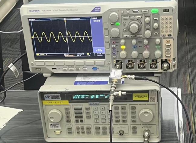
Figure 2: The instrument on the top is MDO 3024, and the one at the bottom is HP 33250A

A simple T-adapter connection is insufficient to capture the reflected signal, since it can simply combine or split the RF signal. Therefore, we acquire a directional coupler (QM-CP1000), which allows us to select the signal coming from the correct path, to properly route the reflected signal from the antenna to the oscilloscope’s receiving channel (see Figure 3). After making these adjustments and overcoming initial challenges, we are finally able to take the measurements as expected.

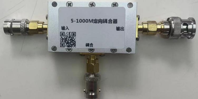
Figure 3: QM-CP1000

3.2. Antenna and system construction

The simplest antenna is a loop antenna, whose length can be easily calculated once the diameter is fixed. To make the antenna, we cut the copper wire to a desired length and shape it into a loop.The process of making the antenna is as follows:

1. To make the wire more circular, we make a cylinder with a diameter of 25.4mm by using household raw material belt, whose cross-sectional circumference is about 79.8mm, as shown in Figure 4.1.

2. We cut a copper wire into a length of 90mm, and wind it on the cylinder to form a ring with a diameter of 25.4mm, as shown in Figure 4.2.

3. We weld the ring to the head of the all-copper BNC KY-50 Insulated Adaptor, as shown in Figure 4.3.

4. A simple antenna is thus made as shown in Figure 4.4.

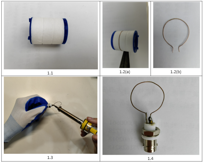
Figure 4: The antenna

Then we build a system composed of the antenna, a one-male-two-female T-adaptor, a three-head coupler, a terminator, an RF analyzer, and a signal generator. As shown in Figure 5, the T-adaptor is connected to the coupler on the output edge. The input edge is connected to the RF analyzer, which receives the reflected signal of the antenna.

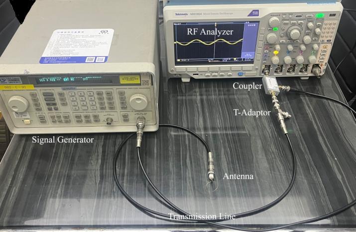
Figure 5: The system

Now we turn to the length of the terminal lines. It is easy to understand that the transmission line connecting the coupling edge to the signal generator does not have a specific length. As for the transmission line between the T-adaptor and the terminator, it has a length of zero meters, given l is equal to the combined length of the terminator and the T-adaptor. As shown in Figure 6, the d value is the distance from the T-Adapter to the antenna tail, and the combined length of the right side of the T-Adaptor and the BNC KY-50 Insulated Adaptorit is about 0.050m. Therefore, the length of the transmission line connecting the antenna and the center of the T-adaptor is 0.983m (= \( 1.033-0.050 \) ).

This problem is actually encountered in our experiment. The first time when we made the transmission lines, we cut them with d and l values. As a result, the data we obtained was skewed from what we had expected, and there was actually no apparent pattern. Being awared of this, we remeasured the length of the two transmission lines and made adjustments accordingly.

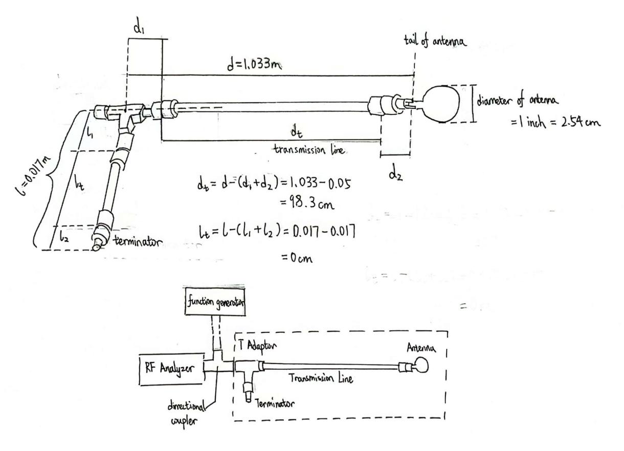
Figure 6: System structure

3.3. Testing

After connecting the system, the generator outputs signals at various frequencies, which are controlled via its interface. Due to the challenges in directly measuring the magnetic field generated by the antenna, we quantify the efficiency of the antenna system by analyzing the reflected signals, which can indicate possible impedance mismatches. This approach is grounded in the principle of energy conservation, as no energy is stored in the transmission lines. We expect the reflected signal to be minimized when the impedance-matching system is functioning correctly, which can be verified through spectral analysis.

For each sample period of \( 4.0×{10^{-6}} \) seconds, the RF analyzer collects the reflected signal (see Figure 7) for 10,000 times evenly and then converts them into a CSV table. This is equivalent to recording the value of power every 1/10,000 of a \( 4.0×{10^{-6}} \) second. The data is then stored on a computer that is connected to the RF analyzer.

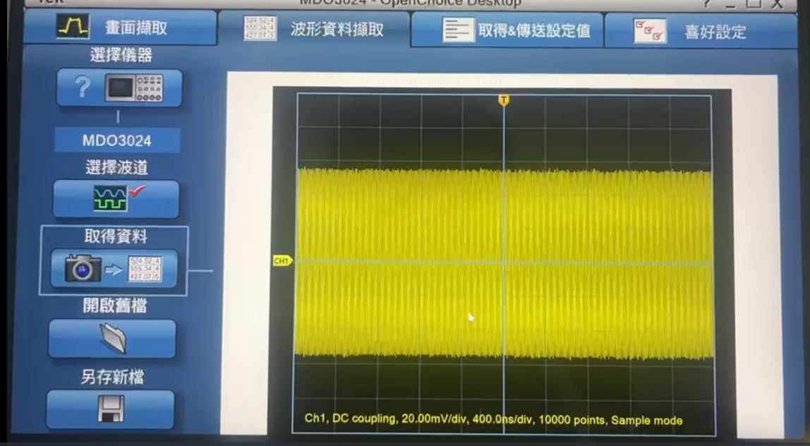
Figure 7: Reflected signal captured on MDO3024

To examine the role of the impedance matching system, we run the test with and without the system, respectively. Considering the relationship between the reflected signal and the output frequency, our tests are made across a range of frequencies at values between 30 and 130 MHz. As indicated in the calculations, we expect the resonance to occur around 80 MHz. Consequently, we perform a fine scan near this frequency. Additionally, potential sidebands might appear farther from the resonant frequency; however, these typically have a much broader bandwidth, allowing for larger scan steps in those regions. 2

4. Data analysis

For the 10,000 power data collected at each sample period at certain frequency, we define the highest one as \( {P_{max}} \) . Figure 8 and Figure 9 give an example of how \( {P_{max}} \) is obtained at a frequency of 80 MHz with and without the antenna, respectively. More specifically, the maximum power reaches 0.074 \( μW \) when there is the antenna, higher than that of 0.056 \( μW \) when there is no antenna.

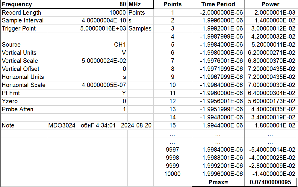
Figure 8: Data at 80 MHz with antenna

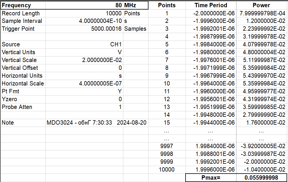
Figure 9: Data at 80 MHz without antenna

Given the expectation and reasoning, we conduct tests at intervals of 1 MHz between 60 and 90 MHz, 5 MHz between 50 to 60 MHz and 90 to 100 MHz, and 10 MHz between 30 to 50 MHz and 100 to 130 MHz. Figure 10 shows \( {P_{max}} \) at all sampled frequencies (40 groups in total) with our experiment. Data collected with antenna are shown in red, and the ones without antenna are shown in blue. The figure clearly demonstrates that \( {P_{max}} \) is stable when there is the antenna but becomes more volatile without it.

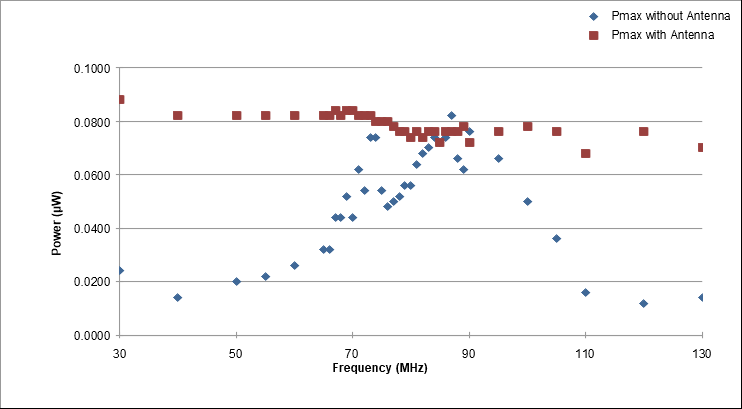
Figure 10: \( {P_{max}} \) with and without antenna

Figure 11 presents the difference between \( {P_{max}} \) with and without the antenna at every identical frequency, which is denoted as \( Δ{P_{max}}(={P_{maxwith antenna}}-{P_{maxwithout antenna}}) \) . We find that \( Δ{P_{max}} \) approaches 0 \( μW \) when the frequency is around 87 MHz (not far from 80 MHz) , which may indicate the occurrence of some systematic errors when the system was constructed. Overall, these features show that the impedance-matching system functions well in the specified interval.

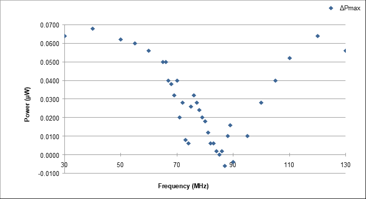
Figure 11: Difference in \( {P_{max}} \)

5. Conclusion

In this project, we explore the fundamental concepts of electromagnetism and impedance matching to optimize signal transmission to a small antenna. This approach is essential for generating a directional magnetic field in a limited space. We apply these principles to design and build a system consisting of a small antenna and a corresponding impedance-matching network, specifically tuned to 80 MHz. The system’s effectiveness is confirmed by measuring the reflected signal from the antenna.

Meanwhile, we observe a discrepancy between the actual impedance matching frequency and the calculated value. This mismatch could be due to several factors, with the most likely one being the inaccuracies in measurements, such as cable length, and the dimensions and material properties of the antenna. Additionally, imperfections in the RF components may also contribute to this issue, as the impedance matching system is highly sensitive, and even minor deviations can cause significant shifts in the peak response.

Moving forward, enhancing precision in dimension measurements is crucial for improving the accuracy of impedance-matching predictions. With a more refined setup and algorithm, this system could be scaled for mass production, providing valuable applications, particularly in laboratory settings. In addition, given the system is currently designed for a fixed frequency, we expect future research to explore the possibility of making the target frequency adjustable. For example, by introducing adjustable components to the coaxial cable or combining passive elements to provide a variable impedance factor, we could easily apply the two equations from the theoretical section to determine the necessary lengths or impedance values. This would enable the creation of an impedance matching system for a given frequency range.

References

[1]. D. J. Griffins, Introduction to Electrodynamics, 4th ed. (PEARSON Education Inc., 2013).
[2]. J. D. Jackson, Classical electrodynamics, 3rd ed. (Wiley, New York, NY, 1999).
[3]. E. Stein and R. Shakarchi, Complex Analysis (Pinceton University Press, 2003).
[4]. N. K. Nikolova, Lecture 12: Loop antennas (2023).
[5]. D. M. Pozar, Microwave Engineering (Wiley, 2012).
[6]. S. Gupta, Z. Hadzibabic, M. W. Zwierlein, C. A. Stan, K. Dieckmann, C. H. Schunck, E. G.M. V. Kempen, B. J. Verhaar, and W. Ketterle, Science Vol.300, pp. 1723-1726 (June 2003).
[7]. C. Chin, A. A. M. Bartenstein, S. J. S. Riedl, J. H. Denschlag, and R. Grimm, Science Vol.305, pp. 1128-1130 (August 2004).
Cite this article
Wang,Z.(. (2025). The Design of An Impedance Matching System with A Small RF Antenna. Applied and Computational Engineering,155,142-152.
Data availability
The datasets used and/or analyzed during the current study will be available from the authors upon reasonable request.
Disclaimer/Publisher's Note
The statements, opinions and data contained in all publications are solely those of the individual author(s) and contributor(s) and not of EWA Publishing and/or the editor(s). EWA Publishing and/or the editor(s) disclaim responsibility for any injury to people or property resulting from any ideas, methods, instructions or products referred to in the content.
About volume
Volume title: Proceedings of CONF-FMCE 2025 Symposium: Semantic Communication for Media Compression and Transmission
© 2024 by the author(s). Licensee EWA Publishing, Oxford, UK. This article is an open access article distributed under the terms and
conditions of the Creative Commons Attribution (CC BY) license. Authors who
publish this series agree to the following terms:
1. Authors retain copyright and grant the series right of first publication with the work simultaneously licensed under a Creative Commons
Attribution License that allows others to share the work with an acknowledgment of the work's authorship and initial publication in this
series.
2. Authors are able to enter into separate, additional contractual arrangements for the non-exclusive distribution of the series's published
version of the work (e.g., post it to an institutional repository or publish it in a book), with an acknowledgment of its initial
publication in this series.
3. Authors are permitted and encouraged to post their work online (e.g., in institutional repositories or on their website) prior to and
during the submission process, as it can lead to productive exchanges, as well as earlier and greater citation of published work (See
Open access policy for details).