1. Introduction

1.1. Background

The development of causal inference as a core methodology linking statistics and decision science has gone through three paradigm leaps. The early stages were based on Fisher's randomized controlled trials (RCTs) [1] and Rubin's potential outcomes framework [2] as the cornerstone of the gold standard system of evidence generation. However, the high cost and ethical constraints of RCTs gave rise to observational research methods, and the propensity score matching (PSM) method proposed by Rosenbaum & Rubin [3] presented an early option for fitting experimental studies from observational studies. PSM has shown reliable performance only in low-dimensional scenarios, but cannot be adapted to high-dimensional, complex scenarios with control of confounders [4]. Pearl's structural causal model [4] formalizes the intervention effect through the do-operator, suggesting a reliable way of screening for confounders based on causal diagrams, which gives the causal model a more structured character. However, the pre-construction of causal graphs relies heavily on a priori knowledge of the domain. It was not until the introduction of machine learning techniques that broke through the curse of dimensionality and the bottleneck of non-linear modelling of traditional methods. Currently, the integration of causal inference and machine learning presents multiple paths: as a tool to improve estimation accuracy, e.g., the orthogonalization mechanism of DML [5], and as a subject to drive causal representation learning, e.g., counterfactual generation of CausalGAN [6] and so on.

1.2. Research topic

This study systematically sorts out machine learning-driven causal inference methods and constructs a three-dimensional classification framework to provide a detailed division of tasks in different scenarios. This study categorizes these causal inference methods from a more nuanced perspective: (1) from the type of task, whether it is a quantitative estimation of causal effects or discovery of causal structure; (2) from the characteristics of the task data, e.g., whether it is temporal type of data or high-dimensional and complex data; and (3) from the theory of the algorithms, the theoretical framework of the algorithms that allow them to implement causal inference, in terms of the way the algorithms are used. And the perspectives of (1) and (2) will provide guidance for constructing the algorithm evaluation system, the decision matrix.

The core goal is to establish a three-dimensional selection criterion of "algorithm-scenario-evaluation" to solve the problem of fragmentation of the evaluations in the current research [5], and hopefully to provide researchers with a reference guide for model selection.

1.3. Research methodology

Systematically combing mainstream causal inference methods combining machine learning (deep learning/deep representation learning), evaluating the performance of algorithms through a multi-indicator evaluation framework on the basis of which a decision matrix is constructed: (1) Establishment of the evaluation system: giving the corresponding priority relationship between the evaluation indicators of different algorithms and the corresponding domains, and what domains should be given priority to what indicators. (2) Decision Matrix Establishment: Based on the evaluation system, construct the decision matrix, and select suitable algorithms according to different domain requirements and data characteristics. (3) Benchmarking analysis: IHDP open standard dataset cross-model comparison to verify the universality of the decision matrix. The main indicators include PEHE (individual processing effect error), ATE deviation, do-SHAP causality interpretability.

1.4. Research contribution

This study makes innovative contributions across three dimensions: Theoretically, it establishes a systematic overview of machine learning-driven causal inference algorithms, providing a comprehensive framework for the field; Methodologically, it develops a multi-criteria decision matrix for causal model selection, enabling scientifically grounded decision-making by holistically weighing algorithmic properties, application scenarios, and task requirements; Practically, it validates the framework’s universality through a case study in classical medical domains, demonstrating its operational feasibility and effectiveness in real-world settings. Together, these contributions form an integrated research cycle spanning theoretical foundation, methodological innovation, and empirical validation.

2. Literature review

2.1. Early-aged statistical methods

Beginning with R.A. Fisher's introduction of the RCT [1], statistics formally began to deal with the problem of causal inference. The central task was to control for confounders. Fisher did this by directly equalizing confounders across subgroups through human intervention. However, this is not a very generalizable approach because the researcher often cannot decide whether to intervene or not. So Philip proposed the instrumental variable (IV) [7], which now seems to be the so-called mediating variable, with the help of which the effect exerted by the intervention is obtained indirectly. Other researchers have tried to control for confounders in this way by including in the regression analysis all the factors considered likely to be confounders under the current observation. Obviously regression analysis cannot deal with unanticipated factors, and Cochran [8] modeled the effect of the RCT through the idea of stratification, making the treatment and control groups comparable within each stratum. Such an approach creates problems that are difficult to deal with once there is too much confounders.

2.2. Improvement of early-aged statistical methods

2.2.1. Potential outcomes framework

Rubin gives concepts in his theory that are used to this day. Rubin gives a formal mathematical expression of intervention in his doctrine and gives definitions of observed, potential, and counterfactual outcomes based on the definition of intervention. The intervention-based definition divides all the variables in the character into pre-intervention and post-intervention variable

According to the association of the front and back pieces of causality. From Rubin's theoretical framework it is possible to derive a mathematical expression for the so-called causal effect:

\( ATE=E[Y(W=1)-Y(W=0)] \) (1)

The potential causation framework [2] makes three important assumptions: (1) The stable unit intervention value assumption. In layman's terms, this means that there is independence between each of the smallest object-units in causal inference; each intervention takes only one form and leads to only one fixed outcome, and there will not be multiple outcomes. (2) Ignorable assumption. In layman's terms, the significance of this assumption is that for a given unit of the pre-intervention variable, the allocation strategy of the different interventions of Akin is considered to be the same. This assumption is the theoretical basis for non-confounding. (3) Positivity. In simple terms, this means that for any pre-intervention variable, the intervention is indeterminate and there is variability. Based on these three assumptions, we can obtain mathematical definitions about all intervention effects:

\( {ITE_{i}}={W_{i}}Y_{i}^{F}-{W_{i}}Y_{i}^{CF}+(1-{W_{i}})Y_{i}^{CF}-(1-{W_{i}}) \) (2)

\( ATE={E_{X}}[E[{Y^{F}}|W=1,X=x]-E[{Y^{F}}|W=0,X=x]] \)

\( =\frac{1}{N}\sum _{i} ({Y_{i}}(W=1)-{Y_{i}}(W=0))=\frac{1}{N}\sum _{i} {ITE_{i}} \) (3)

\( ATT={E_{{X_{T}}}}[E[{Y^{F}}|W=1,X=x]-E[{Y^{F}}|W=0,X=x]] \)

\( =\frac{1}{{N_{T}}}\sum _{\lbrace i:{W_{i}}=1\rbrace } ({Y_{i}}(W=1)-{Y_{i}}(W=0))=\frac{1}{{N_{T}}}\sum _{\lbrace i:{W_{i}}=1\rbrace } {ITE_{i }} \) (4)

\( CATE=E[{Y^{F}}|W=1,X=x]-E[{Y^{F}}|W=0,X=x] \)

\( =\frac{1}{{N_{x}}}\sum _{\lbrace i:{X_{i}}=x\rbrace } ({Y_{i}}(W=1)-{Y_{i}}(W=0))=\frac{1}{{N_{x}}}\sum _{\lbrace i:{X_{i}}=x\rbrace } {ITE_{i}} \) (5)

Taken together, causal inference in this framework centers on estimating the average potential intervention outcome and control outcome on a subgroup. And this estimate is affected by confounding variables. Thus, the difficulty of the task migrates to how to eliminate the effects of confounders. To eliminate the effect of confounding factors, researchers have worked out different solutions. One of them is to address the selection bias induced by the confounders by fitting an unbiased subgroup and eliminating the confusion. This category is represented by methods such as propensity score matching, inverse probability weighting, and methods based on representation learning. The other class of methods deals directly with biased data and corrects the results after obtaining them. This class is represented by meta-learning methods. We will continue to refer to these methods later in this discussion.

Rubin's [2] causal model linked individual potential outcomes \( {Y_{i}}(T) \) to individual treatments \( { T_{i}} \) and individual confounders \( {X_{i}} \) to formalize the causal effects of RCT through the potential outcome framework, which provides theoretical underpinning for RCT, and serves as a theoretical framework that guides a series of subsequent new approaches to causal inference, providing them with an explanatory basis.

2.2.2. Structural causal modeling

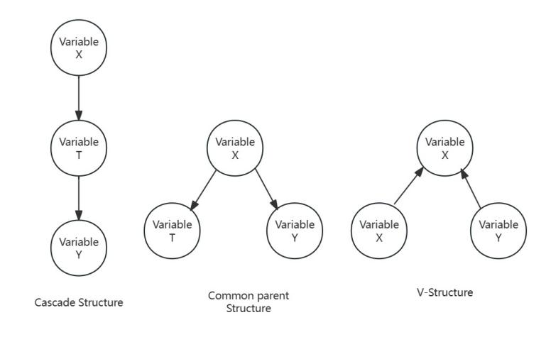
Figure 1: Three basic structures of the Structural Causality Model

Pearl [4] developed a more structured and understandable theory, the Structural Causality Model. Pearl improved on Rubin's theory. It can be found that Rubin's theory can only change one variable at a time and only observe changes in a single variable. The key idea is to introduce the prior knowledge of domain experts to construct a priori conditionally independent distributions simplifying the joint distribution. Pearl developed a theory that could handle more variables and be clearer. Specifically, Pearl gives the front-door criterion, back-door criterion, instrumental variables, which are reflected in the DAG as V-structure, common parent structure, and cascade structure as shown in Figure 1. With the d-separation method given by Pearl, researchers can use Bayesian networks to quickly build up model presets. Researchers can use Bayesian networks to quickly build up model presets. However, relationships in Bayesian networks are not equivalent to causal relationships. To truly characterize causal relationships, one also needs to resort to the potential causal framework. Pearl [4] introduced exogenous variables to solve this problem.

Pearl's combines do-calculus with the SCM to formalize intervention effects through the intervention distribution \( P(Y|do(A)) \) , making SCM a clearer demonstration of true causality than SEM, and more rigorously defined.

2.2.3. Comments and evaluation

Rubin and Pearl's theory systematized the theory of causal inference to the point where causal inference became a rigorous discipline. The theories of the two also became the classic theories in the field, continuing to give theoretical justification for subsequent research and providing ideas for subsequent methodological design. However, there are limitations to their approach. Subsequent researchers have encountered different problems along the lines of Rubin and Pearl's approach when dealing with more complex tasks with larger amounts of data. For example, the PSM approach was not adapted to the later, more complex scenarios, and Stuart's [9] meta-analysis showed that PSM's balancing efficiency declined by 37%-52% (95% CI: 28.6-61.3) when confounders’ dimensionality exceeded 30, and it was unable to deal with unobserved confounders variables. And Hernán [10] found that structural equation modelling parameter estimation errors amounted to 68.7% (vs DML, p<0.001) when causal maps contained more than five mediating variables, exposing the vulnerability of models to be set up incorrectly in advance. These prompted a revolution in methodology.

2.3. Combining causal inference methods with machine learning

2.3.1. Combining causal inference with classical machine learning

Early causal inference combined with classical machine learning algorithms was designed to address the limitations of traditional statistical methods that perform poorly in high-dimensional situations and non-linear relationships, so the idea was to first utilize the machine learning algorithm's ability to process high-dimensional data, and then adapt that machine learning algorithm to have the theoretical characteristics of causal inference: i.e., the ability to efficiently control confounders, and the ability to perform counterfactual inference. Based on the ideas mentioned above, the researcher developed four approaches.

The first one is the extension and generalization of the propensity score model: applying Gradient Boosting Tree (GBM) [11] instead of Logistic Regression to estimate the propensity score, or adopting Generalized Propensity Score Matching (GPSM)[12], the core idea is to extend the previous PSM with machine learning algorithms, so as to make it build up the propensity score estimation of higher accuracy in more high-dimensional scenarios, clearly an inheritance of the potential causal framework. Simply put, GPSM has three processes. The first step is to calculate the probability that an individual is assigned to a treatment group given the covariates and to give a criterion (propensity score) indicating the similarity of these individuals to the treatment group; in the second step, different algorithms are used to obtain the samples of the control group that are nearest neighbors to the treatment group; and in the third step, the ‘neighbors’ obtained in the second step are computed to obtain the Treatment effects.

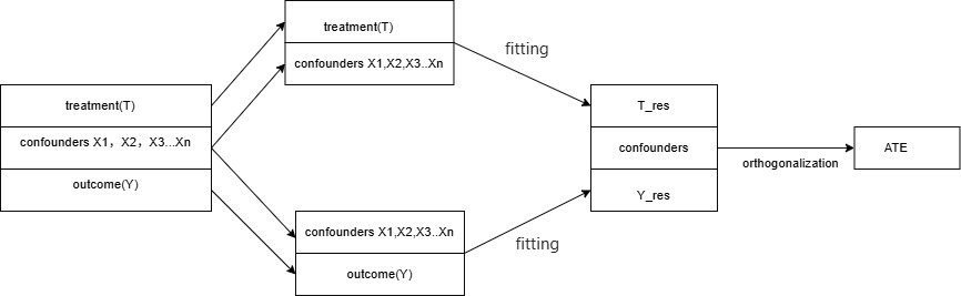
Figure 2: The double machine learning method

The second method is another inheritance of the potential outcome framework what is known as the double robust method. Several typical algorithms are derived from this approach: Targeted Maximum Likelihood Estimation (TMLE) [13] avoids bias by correcting the initial estimation with an influence function, which has the advantage of not only utilizing the information within the data to estimate the parameters, but also by the additional "targeting" of the It has the advantage of not only using the information within the data to estimate the parameters, but also through additional "targeting" to adjust the estimate for specific parameters, which makes it highly robust. Augmented Inverse Probability Weighting (AIPW) [14] combines inverse probability weighting and outcome regression to synthesize the propensity score model and the outcome model, which makes it possible for as long as one of the models is correct, the then the estimation will be unbiased. We take DML as an example. As shown in Figure 2, it can be seen that both dual robust methods require the fitting of two models. The difference lies in how the effects of fitting the two models are handled. Double Machine Learning (DML), on the other hand, uses orthogonalization to process the results. DMLs [5] idea of eliminating confounders bias was achieved by fitting the treatment model and the outcome model in two stages and orthogonalizing the residuals of the two fits.

The third method heterogeneous treatment effect model is specifically designed to estimate treatment effects on subgroups and still based on potential causal framework. With the design idea of heterogeneity treatment, researchers have developed different approaches: optimizing the splitting rules of random forests to obtain causal forests. Meta-learners provide diverse choices, giving frameworks, such as S-learner, T-learner, etc., where researchers reduce the bias and variance by efficiently combining classical machine learning algorithms. Similarly, meta-learners is a framework. Different machine learning algorithms can also be chosen as per the need. But in a nutshell, in this framework, the formula for calculating ATE, ITE is as follows:

\( τ=E\lbrace Y(1)-Y(0)\rbrace \) (6)

\( τ({x_{i}})=E({Y_{i}}(1)-{Y_{i}}(0)|{x_{i}})=E(E(Y|T=1,{x_{i}})-E(Y|T=0,{x_{i}})) \) (7)

In this study, the classic T-learner was chosen as an example to explain the practice of meta-learners. The central task was to fit the expectations of the two outcome variables for the treatment and control groups. That is, the following expression:

\( \begin{array}{c} {μ_{1}}({x_{i}})≔E(Y|T=1,{x_{i}}) \\ {μ_{0}}({x_{i}})≔E(Y|T=0,{x_{i}}) \end{array} \) (8)

And Bayesian Additive Regression Trees ( BART) [15] can fit quite complex data structures using additive combinations of regression trees, which has a unique advantage when facing complex scenarios.

Unlike the first three methods, the fourth method inherits the idea of SCM. The fourth approach is an inheritance and extension of the classical theory of instrumental variables. Such an idea can be combined with many previously summarized algorithms, such as Double Machine Learning (DML) with IV, BART-IV, random forest-IV, and so on. Combining the idea of instrumental variables allows the powerful predictive ability of these machine learning to be utilized.

2.4. Fusion of causal inference and deep learning

As machine learning-driven causal inference methods have come to fruition in a wider range of domains, researchers have applied causal inference to datasets with larger data volumes and more complex features. This has led to difficulties in combing causal structures with a priori knowledge, and the sheer volume of data has made feature engineering extremely difficult. The researcher turned to deep learning for help. Firstly, with deep learning's effective capture of complex interaction effects between treatment variables and confounders, researchers can generate counterfactual predictions by learning dataset’s features. CEVAE [16] applies the idea of adversarial generation to causal inference for the first time. It uses VAE to model potential confounders, thus providing more accurate estimates of causal effects in the presence of unobserved confounders. After this, the idea of adversarial generation was also applied to causal inference. GANITE [17] revolutionized causal inference by introducing a generator-discriminator architecture that explicitly gave counterfactual results. Each of these two approaches derives many variants based on specific task scenarios, demonstrating the potential of deep learning in the field of causal inference. Secondly, deep representation learning also shows advantages in removing confounders effects. This approach typically learns common features between data from different variables in a dataset, and then takes a different approach to applying those features. For example, TARNet is like adding a simple feature sharing representation layer to T-learner's feature layer. Based on TARNet, in order to more accurately balance the distribution of the trained and control groups in the representation space, CFRNet [18] corrects the distribution distance measuring the trained and control groups by adding an extra loss on top of the TarNet's loss, which is called integral probability metrics (IPM). In order to more accurately balance the distribution of the trained and control groups in the representation space, we can add an additional loss to the TARNet's loss to correct the distance between the distribution of the trained and control groups, which is called integral probability metrics (IPM). DragonNet [19] uses this feature value to eliminate the confounders effect by redistributing data from different treatment groups with the help of the idea of propensity score matching; and TARNet [20] models the treatment group and the control group separately, separating the shared representation and the treatment effect. Thirdly, the framework of instrumental variable approach has always been advantageous, which promotes researchers to apply deep learning methods to the framework of instrumental variables. The specific method involved may simply be the use of deep learning as an alternative to traditional methods to study correlation, combined with the theory of causal inference for validation, so it will not be repeated here. The most important thing I would like to mention at this stage of this study is time-series causal inference. Causal inference on time-series data is a theoretical creation. Previous methods have tended to address static problems by design and failed to address dynamic interventions with long-range dependencies. Time-series data is different from the general static data of a certain time cross-section, the premise of independent and homogeneous distribution is no longer valid; in order to deal with autocorrelation and dynamic changes in time-series data, the structure of convolution and recursion provides a solution to capture time-series dependencies. Convolutional Neural Network (CNNs) for the first time incorporate the method of Recurrent Neural Networks (RNNs), and the recursive structure helps to capture temporal dependencies. Subsequent researchers applied the classical conclusions of SCM to CRN, enhancing its ability to face complex scenarios. Dynamic-TE [21], on the other hand, marks a shift from causal effect estimation at a single point in time to multi-stage dynamic treatment of effect estimation, which captures interactions between different points in time through staged modelling of the treatment effect and supports long-term effect analysis.

2.5. Causal discovery & automated reasoning

With methodological advances, researchers realized that causal structures predicated on a priori knowledge could not be entirely factual. Therefore, attempts have been made to use algorithms to autonomously uncover causal structures from data. This gave rise to causal inference, which, unlike all the previously mentioned methods, has the core tasks of causal structure learning, causal direction identification, hidden variable handling and dynamic causal modelling, and is no longer about eliminating confounders and counterfactual reasoning. Causal discovery has different ideas, but they all inherit the idea of structural causal modeling. Researchers naturally thought of conditional independence testing, and on this idea they invented the PC [22] algorithm and extended the FCI [23] algorithm that can deal with hidden variables. However, the computational complexity of such a method is too high, and it is not suitable for larger datasets; in order to improve such a problem, researchers try to search for the causal graph structure with the highest score through a scoring function, but such an algorithm is often caught in the problem of local optimality; for this reason, the method based on gradient optimization is proposed, and the accuracy of the method and the ability to capture complex scenarios are also greatly improved. Among them, DAG-GNN [24] combines graph neural networks and causal discovery to show excellent causal structure learning ability [24].

3. Evaluation framework establishment

3.1. Multi-dimensional evaluation matrix

There are multiple metrics for assessing the success of a causal inference task. This study will sort through these metrics to give an evaluation matrix for different scenarios.

Table 1: Multi-dimensional evaluation matrix

As Table 1 summarizes, this study briefly summarizes the core needs, priority assessment metrics and time-sequential relevance of causal inference in common domains. Industrial applications and basic causal research need to focus on temporal dynamic causation, such as fault diagnosis, temporal causal discovery, etc., and the priority evaluation indexes include dynamic AUUC (long-term benefit assessment) and temporal consistency error (stability of multi-stage effects); other fields (e.g., healthcare, business decision-making) focus on static causal effects, and the indexes focus on the precision of individual or group effects (e.g., PEHE, Qini coefficient). The following are some of the indicators used in the study. Generic indicators (e.g., Structural Hamming Distance, E-Value) are applicable to all domains, but time-series scenarios need to be extended with dynamic versions. The selection of metrics is driven by "core requirements", e.g., medical domains emphasize confounders control (E-Value), industrial applications rely on causal structure identification (Structural Hamming Distance).

3.2. Construction of decision-making method

Table 2: Metics of the decision-making method

As Table 2 shows, this matrix is based on two core dimensions, task type and data characteristics, to provide researchers with a quick reference from problem definition to method landing. Task type determines the objectives (e.g., individual effects, causal discovery), and data characteristics constrain the method selection (e.g., high-dimensional, time-series, unstructured). Methods that cover different implementation ideas of causal inference and combine different AI algorithms are covered, and methods mentioned in previous literature reviews are also addressed.

3.3. Testing of decision-making methods

3.3.1. Application of standard datasets in healthcare

In this study, the classical dataset IHDP is selected to complete the validation of the algorithm selection matrix. The IHDP dataset is a semi-synthetic dataset used to investigate the causal effect of "expert home visits" (a binary treatment variable) on "infant cognitive test scores" (a continuous outcome variable). The raw data were constructed based on a randomized controlled trial, but were biased to remove part of the intervention group to simulate selection bias in observational studies. The core task is to estimate the average treatment effect (ATE), i.e., the average impact of home visits on cognitive scores. The IHDP contains 747 samples (139 in the intervention group and 608 in the control group) and contains 25 confounders (e.g., infant birth weight, mother's age, education level, etc.) covering both numerical and categorical characteristics. The IHDP contains 747 samples (139 in the intervention group and 608 in the control group) and contains 25 covariates (e.g., infant birth weight, mother's age, education level, etc.) covering both numerical and categorical characteristics. The main processing difficulties are: (1) containing 25 potential confounders with possible redundant features (e.g., highly correlated indicators of maternal and infant health. (2) Selection bias: the intervention group sample was biasedly screened, resulting in an uneven distribution of confounders between the treatment and control groups (e.g., a higher proportion of low-birth-weight infants in the intervention group) (3) Unobserved confounders: the data did not explicitly include all confounders variables (e.g., household economic status), and relied on robustness methods or sensitivity analyses.

3.3.2. Ihdp processing analysis

Combining the previous analyses of the characteristics of the IHDP dataset, based on the algorithmic decision matrix mentioned earlier, we can get the deep learning methods used by the CEVAE, CFRNet, BART and DML frameworks, which should all be selected according to the idea of the decision matrix. The processing results of these methods are compared with other methods as follows. This comparison contains the methods used by other researchers as well as the processing methods added for use in this study.

Summarizing the results of other researchers' implementations and ours in Table 3, a comparison reveals that the processing of these methods is roughly in line with our expectations. Taken together CFRNet is in the best position, with excellent performance in both metrics. The rest of GANITE, BART, CEVAE, and DML (using MLP) show little difference in performance; while Causal Forest and kNN are the worst performers, with both metrics performing poorly. It basically confirms that our algorithmic decision matrix.

Table 3: Summary of the effects of processing the IHDP dataset

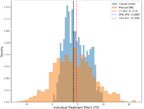
Figure 3: Distribution of ITE for CausalForestDML and DML with MLP

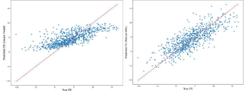
Figure 4: Mapping of processed ITE to actual ITE for two DML algorithms

Figure 3 and Figure 4 show the specific processing effect images of the two DML algorithms added for use in this study, this is the result of the processing of this study using conventional CausalForestDML and DML using MLP as the fitting algorithm. The DML algorithm using MLP has highest accuracy (smallest \( {ϵ_{\lbrace ATE\rbrace }} \) ), and the prediction points are closer to the ideal 45° demarcation line in the prediction of ITEs (smaller \( \sqrt[]{{ϵ_{PEHE}}} \) ). The DML using MLP also demonstrates a stronger ability to capture heterogeneity effects in the distribution of ITEs.

4. Discussion

4.1. Advantages of current methods

Existing causal inference methods show diverse advantages in different scenarios. Experimental causal inference provides unbiased estimates of causal effects through randomized experiments and is the gold standard for assessing causality, but its application may be limited by ethical or cost constraints. Methods such as propensity score matching (PSM) and instrumental variable methods in observational studies provide alternatives for situations where randomized experiments cannot be implemented: PSM reduces selection bias by matching similar individuals, and instrumental variable methods are effective in addressing endogeneity problems caused by unobserved confounders. In recent years, causal inference methods incorporating machine learning (e.g., CFRNet, Causal Forests, and GANITE) have further improved the ability to deal with high-dimensional and complex data, and have significantly improved the precision of estimating heterogeneous treatment effects. In addition, Double Robust Methods (DRMs) combine the advantages of propensity score and outcome regression models, where a consistent causal effect estimate can be obtained with one of the two models correctly specified, a property that enhances the robustness and applicability of the methods. Causal discovery algorithms (e.g., PC algorithm, GIES, and LiNGAM), on the other hand, automatically infer the causal structure among variables from the data, providing a powerful tool for exploring unknown causal relationships, which is a unique advantage especially in the absence of a priori knowledge. Time-series causal inference algorithms for time-series data (e.g. Granger causality analysis, dynamic causal modelling and deep learning-based time-series causal inference methods) capture causal relationships between variables over time, and are applicable in areas such as finance, climate science and neuroscience. Together, these methods form a rich and complementary toolbox for causal inference, driving a wide range of applications of causality research across multiple disciplines.

4.2. Existing problems and challenges

Each of the causal inference methods mentioned above has its own unique strengths, but they also each have certain limitations. All of the algorithms that have inherited the idea of instrumental variables need to find a valid instrumental variable that only indirectly affects the outcome variable by affecting the treatment variable, and how to choose such a variable is the key to solving the problem; if the wrong variable is chosen, then the results will be very different from the real situation. Dual robustness methods, while providing a way to increase robustness, still rely on the premise that at least one model (either the propensity score model or the outcome regression model) is correctly specified, and if both models are incorrectly specified, this may lead to a loss of efficiency or other problems even if an error in either model does not affect the consistency of the final estimates. For time-series causal inference algorithms, such as Granger causality analysis, although it relies on predictive power in time-series data to infer causality, this is not equivalent to true causality because it cannot rule out common external influences and because traditional time-series causal inference methods may perform poorly for complex nonlinear dynamic systems. Causal discovery algorithms infer causal structure primarily based on statistical associations, and thus may have difficulty distinguishing between direct causality and spurious correlation due to potential confounders, while most such algorithms assume that the data generation process follows a particular form, which may not be applicable to all types of data or application scenarios. These algorithms have limitations or rely on assumptions that may not be true.

5. Conclusion

This study comprehends the development history of causal inference methods, and systematically combs the classical and mainstream methods in different periods, discusses in detail the ideological framework, suitable application scenarios, and advantageous characteristics of different methods; explores what indexes should be prioritized to measure the effect of algorithms in different task scenarios, and establishes an algorithmic selection recommendation matrix based on the foregoing, with a view to providing a quick and easy way for less-skilled researchers to Select the corresponding algorithm according to the task scenarios, and selected the classical dataset IHDP to validate our selection matrix, and get better results after validation. There are some areas for improvement in the current study: in the future, more datasets with different task requirements and data characteristics should be added to do more validation of the algorithm selection matrix and verify its generality; in addition, this study pays insufficient attention to some cutting-edge causal inference methods, and does not have a broad enough horizon for predicting future prospective studies.

The future development of causal inference will show the following trends: firstly, more advanced algorithms will provide stronger computational fitting capabilities for the theoretical framework of causal inference, while dynamic causal inference (e.g., temporal causal modelling, causal decision-making in reinforcement learning) will address the problem of multiple interventions and long-term effects in complex systems, and will be more widely applied in more fields. Second, the combination of federated learning frameworks and differential privacy techniques (federated causal inference) will promote privacy-preserving analyses of multi-source data under the current trend of distributed computing becoming mainstream, while fairness-constrained causal models will ensure unbiased estimation in different groups and enhance the ethical compliance of the models. Third, causal inference will take on an automated and instrumented character in the future, with companies such as Google inheriting and encapsulating key algorithms for causal inference into open-source tool libraries, lowering the threshold of causal inference use and supporting rapid application by non-experts in healthcare, policy, and other fields. Overall, causal inference will be more relevant to real-world specific problems in the future (dynamic, complex qualities), more instrumental and low-threshold, and becoming a more general basic tool.

References

[1]. Box, J. F. R.A. Fisher and the Design of Experiments, 1922–1926. Am. Stat. 1980, 34 (1): 1–7.
[2]. Rubin, D. B. Estimating Causal Effects of Treatments in Randomized and Nonrandomized Studies. J. Educ. Psychol. 1974, 66 (5):688–701.
[3]. Rosenbaum, P. R.; Rubin, D. B. The Central Role of the Propensity Score in Observational Studies for Causal Effects.
[4]. DAWID, A. P. Causal Diagrams for Empirical Research: Discussion of "Causal Diagrams for Empirical Research" by J. Pearl. Biometrika, 1995, 82 (4): 689–690.
[5]. Chernozhukov, V.; Chetverikov, D.; Demirer, M.; Duflo, E.; Hansen, C.; Newey, W.; Robins, J. Double/Debiased Machine Learning for Treatment and Structural Parameters. Econom. J. 2018, 21 (1), C1–C68. https://doi.org/10.1111/ectj.12097.
[6]. Hill, J. L. Bayesian Nonparametric Modeling for Causal Inference. J. Comput. Graph. Stat. 2011. https://doi.org/10.1198/jcgs.2010.08162.
[7]. The Tariff on Animal and Vegetable Oils. Philip G. Wright | Journal of Political Economy: Vol 38, No 5. https://www.journals.uchicago.edu/doi/abs/10.1086/254144 (accessed 2025-04-15).
[8]. Cochran, W. G.; Chambers, S. P. The Planning of Observational Studies of Human Populations. J. R. Stat. Soc. Ser. Gen. 1965, 128 (2): 234–266.
[9]. Stuart, E. A. Matching Methods for Causal Inference: A Review and a Look Forward. Stat. Sci. Rev. J. Inst. Math. Stat. 2010, 25 (1), 1–21. https://doi.org/10.1214/09-STS313.
[10]. Causal Inference: What If (the book) — Miguel Hernán. https://miguelhernan.org/whatifbook (accessed 2025-04-15).
[11]. Friedman, J. H. Greedy Function Approximation: A Gradient Boosting Machine. Ann. Stat. 2001, 29 (5), 1189–1232.
[12]. Abadie, A.; Imbens, G. W. Large Sample Properties of Matching Estimators for Average Treatment Effects. Econometrica 2006, 74 (1): 235–267.
[13]. Van Der Laan, M. J.; Rose, S. Targeted Learning: Causal Inference for Observational and Experimental Data; Springer Series in Statistics; Springer: New York, NY, 2011.
[14]. Van Der Laan, M. J.; Rose, S. Targeted Learning: Causal Inference for Observational and Experimental Data; Springer Series in Statistics; Springer: New York, NY, 2011.
[15]. BART: Bayesian additive regression trees. https://projecteuclid.org/journals/annals-of-applied-statistics/volume-4/issue-1/BART-Bayesian-additive-regression-trees/10.1214/09-AOAS285.full (accessed 2025-04-15).
[16]. Louizos, C.; Shalit, U.; Mooij, J. M.; Sontag, D.; Zemel, R.; Welling, M. Causal Effect Inference with Deep Latent-Variable Models. In Advances in Neural Information Processing Systems; Curran Associates, Inc., 2017; Vol. 30.
[17]. Yoon, J.; Jordon, J.; Schaar, M. van der. GANITE: Estimation of Individualized Treatment Effects Using Generative Adversarial Nets; 2018.
[18]. Chauhan, V. K.; Molaei, S.; et al. Adversarial De-Confounding in Individualised Treatment Effects Estimation. In Proceedings of The 26th International Conference on Artificial Intelligence and Statistics; PMLR, 2023; pp. 837–849.
[19]. Shi, C.; Blei, D.; Veitch, V. Adapting Neural Networks for the Estimation of Treatment Effects. In Advances in Neural Information Processing Systems; Curran Associates, Inc., 2019; Vol. 32.
[20]. Shalit, U.; Johansson, F. D.; Sontag, D. Estimating Individual Treatment Effect: Generalization Bounds and Algorithms. In Proceedings of the 34th International Conference on Machine Learning; PMLR, 2017; pp. 3076–3085.
[21]. Ghosh, S.; Feng, Z.; Bian, J.; Butler, K.; Prosperi, M. DR-VIDAL-Doubly Robust Variational Information-Theoretic Deep Adversarial Learning for Counterfactual Prediction and Treatment Effect Estimation on Real World Data. In AMIA Annual Symposium Proceedings; 2023; Vol. 2022, pp. 485.
[22]. Spirtes, P.; Glymour, C. N.; Scheines, R. Causation, Prediction, and Search; MIT Press, 2000.
[23]. An Algorithm for Causal Inference in the Presence of Latent Variables and Selection Bias | Computation, Causation, and Discovery | Books Gateway | MIT Press. https://direct.mit.edu/books/edited-volume/4789/chapter-abstract/218906/An-Algorithm-for-Causal-Inference-in-the-Presence?redirectedFrom=fulltext (accessed 2025-04-15).
[24]. Chen, L.-C.; Papandreou, G.; Kokkinos, I.; Murphy, K.; Yuille, A. L. Semantic Image Segmentation with Deep Convolutional Nets and Fully Connected CRFs. arXiv June 7, 2016.
Cite this article
Xiao,J. (2025). Machine Learning-driven Causal Inference Methods: Progress, Evaluation and Multi-Domain Applications. Applied and Computational Engineering,160,128-141.
Data availability
The datasets used and/or analyzed during the current study will be available from the authors upon reasonable request.
Disclaimer/Publisher's Note
The statements, opinions and data contained in all publications are solely those of the individual author(s) and contributor(s) and not of EWA Publishing and/or the editor(s). EWA Publishing and/or the editor(s) disclaim responsibility for any injury to people or property resulting from any ideas, methods, instructions or products referred to in the content.
About volume
Volume title: Proceedings of CONF-SEML 2025 Symposium: Machine Learning Theory and Applications
© 2024 by the author(s). Licensee EWA Publishing, Oxford, UK. This article is an open access article distributed under the terms and
conditions of the Creative Commons Attribution (CC BY) license. Authors who
publish this series agree to the following terms:
1. Authors retain copyright and grant the series right of first publication with the work simultaneously licensed under a Creative Commons
Attribution License that allows others to share the work with an acknowledgment of the work's authorship and initial publication in this
series.
2. Authors are able to enter into separate, additional contractual arrangements for the non-exclusive distribution of the series's published
version of the work (e.g., post it to an institutional repository or publish it in a book), with an acknowledgment of its initial
publication in this series.
3. Authors are permitted and encouraged to post their work online (e.g., in institutional repositories or on their website) prior to and
during the submission process, as it can lead to productive exchanges, as well as earlier and greater citation of published work (See
Open access policy for details).