1. Introduction

Gradient Descent Methods have long been considered as the fundamental methods for deep learning tasks for the reason that the process of all the neural network algorithms finding their way to the solutions is an optimization problem, in which gradient descent is the most widely used method. Different kinds of optimizers exist and each of them is suitable for some certain situation. One of the most popular training techniques for deep neural networks is SGD [1]. Along with strong fundamental theories, SGD achieves receives great popularity for being simple and competitive in various applications. In this paper, the following collection of stochastic and online convex optimization problems are examined: For a convex functions collection \( F(∙,x), x∈X \) where \( F(∙,x):{R^{d}}→R \) and distribution \( P \) on 𝒳, for a closed convex set \( Θ⊂{R^{d}} \) , people wish to find the solution for the following problem:

\( \underset{θϵΘ}{minimize}{{f_{P}}{(θ)≔{E_{P}}{[F(θ,X)]=\int F(θ,x)dP(x)}}} \) (1)

While stochastic gradient methods are good choice for problem (1) for their simplicity and scalability, more contemporary adaptive gradient methods can obtain improved convergence guarantees in situations with non-Euclidean geometries [2,3].

Adaptive gradient method (AdaGrad) is motivated by the high informativeness and discrimination of rare features [4]. By distributing very low rates of learning recurring elements and high rates of learning infrequent characteristics, AdaGrad can perform more informative gradient-based learning by taking the information given by the previous iteration into consideration. Among all the adaptive methods, Adam is the most popular one and is getting more and more attention [5]. It is invented through a combination of AdaGrad and RMSProp (Tieleman & Hinton, 2012) in hope of gathering their advantages and obtaining a algorithm that work well with both sparse gradients and online, non-stationary settings [6]. Adam have been proved to be effective in many optimization problems and taken over as the standard method for training many neural networks.

Nevertheless, Wilson et al. purposed the view that adaptive methods are less generalizable than SGD with momentum facing some deep learning tasks like image classification [7].

To solve this problem, Keskar & Socher improved the generalization performance by proposing SWAT, a strategy that begins with Adam and goes to SGD with a fixed learning rate when reaching the switchover point. The results were pretty good. It achieves a great performance close to SGD and preserves Adam's beneficial properties such as insensitivity to hyperparameters and quick initial response. However, improvements are achieved by using two different algorithms together instead of focusing on the Adam itself [8].

Loshchilov & Hutter investigated the reason why Adam may be outperformed by SGD with momentum, which is the fact that in adaptive methods, L2 regularization is not as effective as weight decay and it just leads to worse results than it does in SGD. Loshchilov & Hutter shows that Adam generalizes much better when decomposing the decoupled weight than L2 regularization for various image recognition datasets [9].

The motivation is to find the best algorithm that can be applied to any case and achieve great performance, which is barely possible since every method is designed for a certain situation. But things become much easier when the options go down to two, Adam and SGD with momentum. By comparing them and try to figure out the reason why Adam can be outperformed may help improve its generalization performance, which means Adam can do a better job than SGD with momentum in the case where it performs poorly without improvement. As a result, practitioners may skip the procedure of trying different algorithms to find the relatively best one in just one case.

The main work of this paper is to further analyze the effect of the inequivalent of L2 regularization and decoupled weight decay mentioned by Loshchilov & Hutter and then show if it is the case in other situations by looking into other deep learning tasks as a complement to Loshchilov & Hutter. In the first experiment this paper use Lenet with both Adam and SGD as optimizers on the popular image classification dataset CIFAR-10, which turns out that Adam outperforms SGD with better accuracy. Then, this paper investigates their differences by looking at Deep Convolution Generative Adversarial Networks, in which this paper chooses fashionMINIST as its dataset [10]. The result show that SGD converges better and achieves better generation of new images.

2. In-equivalence of L2 regularization and weight decay

Now, this section studies the case when adaptive Gradient Methods are not competitive by looking at the most popular Adaptive Gradient Method-Adam and comparing it to SGD with Momentum. Adam has lots of advantages. The execution of this algorithm is simple and straightforward along with great computational efficiency. It doesn’t require much memory space and is suitable for problems with unsteady target or sparse gradient. Besides, the hyperparameters can be explained in an explicit way. However, Adam may not be able to converge or miss the global optimal point. Researches show that one of the reasons why Adam has a poorer performance than SGD with Momentum is that in some deep learning tasks, like image classification, L2 regularization doesn’t work as well as weight decay while they are basically the same in SGD with Momentum [7]. So now this section will try to figure out what exactly generates this difference.

In this paper, it describes that weights decay exponentially as:

\( {θ_{t+1}}=(1-λ){θ_{t}}-α∇{f_{t}}({θ_{t}}) \) (2)

where λ is defined as the rate of the weight decay for each step and \( ∇{f_{t}}({θ_{t}}) \) is defined to be the \( t \) -th batch gradient to be multiplied by a learning rate α. In the case of standard SGD.

Proposition 1 [9]. Standard SGD with a fixed stepsize α runs a fixed distance for batch loss functions \( {f_{t}}(θ) \) with weight decay λ as it runs without weight decay on:

\( f_{t}^{reg}(θ)={f_{t}}(θ)+\frac{{λ^{ \prime }}}{2}‖θ‖_{2}^{2}, with {λ^{ \prime }}=\frac{λ}{α} \) (3)

This shows that for standard SGD, weight decay is equivalent to L2 regularization. Now turn to Adam. As is the intuition, when Adam is optimizing f plus L2 regularization, weights that have the tendency to possess large gradient in f do not get enough regularized as what would happen with decoupled weight decay because the gradient of the regularization and the gradient of \( f \) are scaled at the same time, which results in an in-equivalence of L2 regularization and decoupled weight decay [9].

Proposition 2 [9]. Let \( O \) denote an optimizer that has updates of the form \( {θ_{t+1}}←{θ_{t}}-α{M_{t}}∇{f_{t}}({θ_{t}}) \) when optimizing \( {f_{t}}(θ) \) with weight decay for \( {M_{t}}≠kI(k∈R) \) . Then, for O, no L2 coefficient \( {λ^{ \prime }} \) that can assure running O on batch loss \( f_{t}^{reg}(θ)={f_{t}}(θ)+\frac{{λ^{ \prime }}}{2}‖θ‖_{2}^{2} \) without weight decay is of the same effect with running O on \( {f_{t}}(θ) \) with decay \( λ∈{R^{+}} \) can be found.

Now that this paper has shown that L2 regularization and weight decay are not equivalent in adaptive methods, this paper then shall analyze how this can affect the performance of them. When it comes to SGD, the two mechanisms drive the weights all the way to 0 with the same pace while in adaptive gradient methods with L2 regularization, for both the loss function and the regularizer, the sums of their gradient are rescaled, which is not the case when it comes to the case with decoupled weight decay. With decoupled weight decay, no gradients expect that of the target function is adapted, which guarantees the algorithm to stay effective as the training proceeds. This analysis shows that with L2 regularization both gradients of the target function and the regularization are standardized by their average magnitudes, and therefore weights x with larger average magnitudes are regularized less than other weights. As for decoupled weight decay on the contrary, all weights are regularized at the speeds which are exactly the same, regularizing weights more effectively than what standard L2 regularization does [9].

3. Image Classification

It is believed that adaptive methods achieve poor generalization performance compared to what can be done by SGD with momentum when tested on image classification [7]. So, this section will show if it is always the case by running a simple experiment. In this experiment, this paper does image classification by using one of the most classical Convolutional Neural Networks, Lenet-5.

3.1. Convolutional Neural Network

CNN is a neural network that works especially well with image recognition and classification [11]. The inspiration originated from the biological behaviour of visual cortex, which has a small group of cells sensitive to the visualized area of a certain part [12]. Figure 1. is a simple draw of the structure, which is made up with input layer, convolution layer, pooling layer, fully connected layer and output layer.

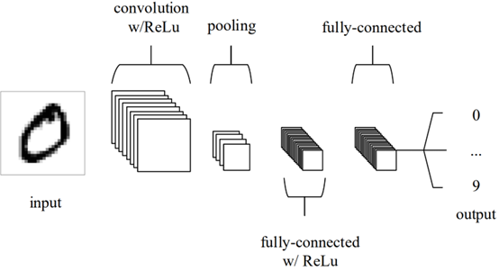
Input layer holds the pixel values of the image just like other ANN. Convolutional layer extracts characteristics of the input image by means of kernel matrix that retains the spatial relations between the pixels. When the number of training parameters is too huge and needs reduction, Pooling layer will down sample the spatial dimensionality of the given input to make the size of the image space smaller. Fully connected layer is the classifier that gets the output of the upper layer and chooses the category that fits the features best. It is also the Muti-Layer Perceptron with Softmax excitation function as the output layer [13, 14].

3.2. Lenet with Adam and SGD on CIFAR-10

Lenet is one of the earliest CNN models that has been put forward. As the final version of Lenet series, Lenet-5 is applied to recognize handwriting numbers by American Bank. All the convolution kernels of Lenet-5 are 5*5 with stepsize 1. It uses mean-pooling as pooling method and Sigmoid as activation function. CIFAR-10 is a dataset consisting of 50000 training images and 10000 testing images, it is used for recognition of some simple items with RGB pictures categorized into 10 classes. The size of the images is 32*32, bigger than 28*28 images in MNIST. Compared to MNIST with handwriting symbols, the images from CIFAR-10 are items from real world, which means the noises are huge and the features are complicated, so it can bring many difficulties for model training. In this experiment, it chooses cross-entropy as loss function and use accuracy of the networks with Adam and SGD on the 10000 test images to see if SGD with momentum can outperform Adam.

In the experiment with SGD as optimizer, it lets learning rate and momentum be 0.001 and 0.9 and train the model for 5 epochs. The result is that after 3 minutes and 59 seconds training, the Lenet-5 model with SGD as its optimizer reaches an accuracy of 59%. In the experiment with Adam on the other hand, it lets learning rate and momentum also be 0.001 and train the model for 5 epochs. The result is that after 4 minutes and 46 seconds training, the Lenet-5 model with SGD as its optimizer reaches an accuracy of 61%.

Table 1. Parameters and Results of the experiment.

As is shown in Table 1, the results of the experiment show that the performances of both SGD and Adam are not so outstanding compared with other models that have reached high accuracy. However, the purpose of this experiment is to show the difference between these two optimizers, so it is simply alright that both of them achieve poor performance. The results show that Adam may takes more time to train the model as is the intuition that Adam may not converge as well as SGD. However, Adam beats SGD with better accuracy, which is against the original thought.

4. Image generation

In this section, it will build a Deep Convolution Generative Adversarial Networks (DCGAN) model to complete Image generation task. Still, it uses both Adam and SGD as optimizers and compare their performance. DCGAN is the original GAN with a improved network structure. Both the Generator and the Discriminator in DCGAN replace the Multi-Layer Perceptron (MLP) in Generative Adversarial Networks (GAN) with a Convolutional Neural Networks (CNN) structure without pooling layer to make sure the whole network is differentiable. The dataset it chooses in this experiment is Fashion-MINST. The dataset contains 10 categories of images, which are t-shirt, trouser, pullover, dress, coat, sandal, shirt, sneaker, bag, ankle boot.

4.1. Deep Convolution Generative Adversarial Networks

DCGAN is composed of two different models, Generative Network and Adversarial Network, or generator and discriminator. The purpose of the generator is to generate fake images that look exactly like the training images. The discriminator, on the other hand, is to check on each image and make the judgement whether it is fake image from the generator or real image from the training set. During the training period, the generator tries to exceed the discriminator by attempting to generate better fake image constantly while the discriminator is to better distinguish fake images from the real ones. The balance strikes when generator can generate the perfect fake images that look exactly like the real ones and the discriminator always categorizes the images from the generator with equal probabilities.

Let \( D(x) \) denote the discriminator and \( D(x) \) denote the generator. z is a random 100-diemsional vector. z is the input of the generator and the output is the image that looks like real images as much as possible. The model trains the generator and discriminator separately. It uses \( log(D(x)+log(D(G(z)))) \) as discriminator’s loss function and \( log(D(G(z))) \) as generator’s loss function.

Notice that, the evaluation of the model is not test accuracy because the samples have no labels. So, unlike what people do in an image classification task, it mainly evaluate the model by how fast the loss decreases in image generation tasks.

4.2. Image generation task on Fashion-MINST

Fashion-MINST was collected to directly replace MINST. The size, number of the images and the number of categories in this dataset are completely the same as those of MINST, which means the switch between these two datasets doesn’t need to change any code. Basically, Fashion-MINST is a more challenging version of MINST.

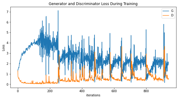
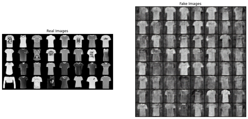
First, it trains the model with Adam as its optimizer. In both Generator and Discriminator, it set learning rate as 0.0002 and betas as (0.5,0.999) and train the model for 5 epochs. The training progress took 46 seconds. The Generator and Discriminator loss during training is shown in figure2. The real images and fake images generated from the Generator are given in figure3.

Then, it trains the model with SGD as its optimizer. In both Generator and Discriminator, it set learning rate as 0.0002 and train the model for 5 epochs. The training progress took 45 seconds. The Generator and Discriminator loss during training is shown in figure 4. The real images and fake images generated from the Generator are given in figure 5.

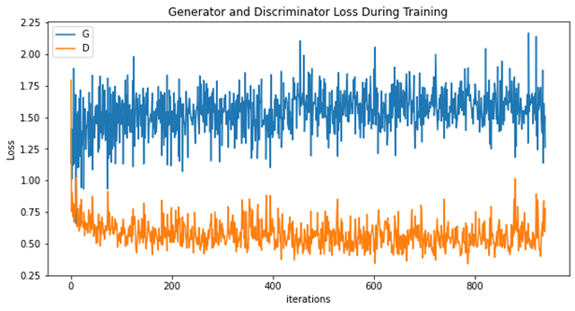
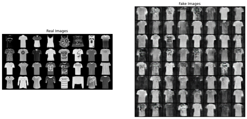
From the results and figures this paper obtain from its experiment, it shows that during the training, it takes the models with both Generator and Discriminator using SGD as optimizer almost the same time to accomplish the training, during which the loss of the model using Adam decreases faster while the loss of the model using SGD goes rather smooth. However, the images generated from the model with SGD is obviously better. The fake image produced by generator with SGD is not only clearer, but also possess more details like stripes or patterns.

From this experiment, it can be seen that in the image generation task, SGD outperforms Adam in terms of the quality of the generative products, which is the main measurement of performance in this task.

5. Conclusion

The experiments in this paper show that, despite previous work demonstrates the fact that SGD can outperform Adam in many of the image classification tasks, Adam still has some little advantages over SGD when classifying images from some dataset. In the experiment with image generation using DCGAN, Adam was outperformed by SGD though Adam is particularly popular in GANs model. From the experiments it can be seen that it is hard to tell which algorithm is better than another even in some certain situation where the theories show that one particular algorithm is supposed to win. In practice, when choosing an optimizer, instead of analyzing the dataset and constraint set, people still tend to try all the optimizers that may achieve great performance and compare them by their results. Lots of work still needs to be done before facing a new deep learning task practitioners can put their foot down and choose one particular optimizer instead of trying them all.

References

[1]. H. Robbins and S. Monro. A stochastic approximation method. Annals of Mathematical Statistics, 22:400–407, 1951.
[2]. Levy D, Duchi J C. Necessary and Sufficient Conditions for Adaptive, Mirror, and Standard Gradient Methods[J]. CoRR, 2019.
[3]. Y. Nesterov. Primal-dual subgradient methods for convex problems. Mathematical Programming, 120(1):261–283, 2009.
[4]. J. C. Duchi, E. Hazan, and Y. Singer. Adaptive subgradient methods for online learning and stochastic optimization. Journal of Machine Learning Research, 12:2121–2159, 2011
[5]. Kingma D P, Ba J. Adam: A method for stochastic optimization[J]. arXiv preprint arXiv:1412.6980, 2014.
[6]. Tieleman, T. and Hinton, G. Lecture 6.5 - RMSProp, COURSERA: Neural Networks for Machine Learning.Technical report, 2012.
[7]. Ashia C Wilson, Rebecca Roelofs, Mitchell Stern, Nathan Srebro, and Benjamin Recht. The marginal value of adaptive gradient methods in machine learning. arXiv:1705.08292, 2017.
[8]. Keskar N S, Socher R. Improving generalization performance by switching from adam to sgd[J]. arXiv preprint arXiv:1712.07628, 2017.
[9]. Loshchilov I, Hutter F. Decoupled weight decay regularization[J]. arXiv preprint arXiv:1711.05101, 2017.
[10]. Radford A, Metz L , Chintala S . Unsupervised Representation Learning with Deep Convolutional Generative Adversarial Networks[J]. arXiv e-prints, 2015.
[11]. Krizhevsky A, Sutskever I, Hinton G E. ImageNet classification with deep convolutional neural networks [J]. Communications of the Acm, 2012, 60(2):2012.
[12]. Kandel E R. An introduction to the work of David Hubel and Torsten Wiesel [J]. Journal of Physiology, 2009, 587(12):2733.
[13]. Quan, Zhang. Convolutional Neural Networks[C]// International Conference on Electromechanical Control Technology and Transportation. 2018.
[14]. O'Shea K, Nash R. An introduction to convolutional neural networks[J]. arXiv preprint arXiv:1511.08458, 2015.
Cite this article
Song,C. (2023). The performance analysis of Adam and SGD in image classification and generation tasks. Applied and Computational Engineering,5,757-763.
Data availability
The datasets used and/or analyzed during the current study will be available from the authors upon reasonable request.
Disclaimer/Publisher's Note
The statements, opinions and data contained in all publications are solely those of the individual author(s) and contributor(s) and not of EWA Publishing and/or the editor(s). EWA Publishing and/or the editor(s) disclaim responsibility for any injury to people or property resulting from any ideas, methods, instructions or products referred to in the content.
About volume
Volume title: Proceedings of the 3rd International Conference on Signal Processing and Machine Learning
© 2024 by the author(s). Licensee EWA Publishing, Oxford, UK. This article is an open access article distributed under the terms and
conditions of the Creative Commons Attribution (CC BY) license. Authors who
publish this series agree to the following terms:
1. Authors retain copyright and grant the series right of first publication with the work simultaneously licensed under a Creative Commons
Attribution License that allows others to share the work with an acknowledgment of the work's authorship and initial publication in this
series.
2. Authors are able to enter into separate, additional contractual arrangements for the non-exclusive distribution of the series's published
version of the work (e.g., post it to an institutional repository or publish it in a book), with an acknowledgment of its initial
publication in this series.
3. Authors are permitted and encouraged to post their work online (e.g., in institutional repositories or on their website) prior to and
during the submission process, as it can lead to productive exchanges, as well as earlier and greater citation of published work (See
Open access policy for details).