1. Introduction

With the continuous growth of global demand for clean energy, wind power, as a vital component of renewable energy, is playing an increasingly important role in achieving carbon neutrality targets and ensuring energy security. In recent years, wind energy has been integrated into power systems at an accelerating rate, becoming a critical force in driving the transition toward green energy. However, due to the combined effects of wind speed uncertainty, regional climate variations, and complex terrain, wind power output exhibits significant nonlinearity, non-stationarity, and strong volatility. These characteristics not only increase the complexity of power grid scheduling but also impose higher requirements on load balancing and market trading strategies. Improving the accuracy and stability of wind power forecasting has thus become a key issue for promoting the efficient integration of renewable energy and ensuring the safe operation of energy systems. High-quality forecasting results can reduce the need for reserve capacity, optimize generation planning, and enhance the pricing power and trading flexibility of wind power enterprises in electricity spot markets, thereby contributing to the construction of a more flexible, efficient, and sustainable power system.

In recent years, a series of emerging deep learning models have demonstrated powerful capabilities in nonlinear time series modeling. However, most existing studies still overlook the interactive effects of trend, periodicity, and perturbation features at different time scales within wind power time series. Particularly in complex scenarios characterized by strong rhythms and frequent structural changes, single-path modeling approaches are prone to prediction bias or failure. To address these challenges, this study constructs a novel forecasting framework—SCiTransformer—by integrating STL decomposition, CNN modules, and the iTransformer architecture. The goal is to achieve multi-scale, multi-modal, and dynamic feature construction for wind power sequences through hierarchical structural decoupling and dynamic modeling mechanisms. Specifically, STL decomposition is employed to extract trend and seasonal patterns, CNN focuses on capturing local abrupt changes and short-term fluctuations, while the iTransformer framework models cross-time-step contextual dependencies and information integration. Through multi-stage fusion, the proposed model collaboratively extracts trend features, local short-term variations, and long-term dependencies from wind power data, significantly enhancing forecasting accuracy and generalization ability. Empirical validation on multiple real-world wind farm datasets demonstrates the model’s robust performance under conditions of complex inputs, low signal-to-noise ratios, and forecasting delays. The research results are expected to provide a theoretical foundation and practical support for optimizing wind farm operations, enabling intelligent grid dispatch, and building green energy trading mechanisms.

2. Literature review

2.1. Applications of machine learning in time series forecasting

In the task of wind power forecasting, traditional machine learning methods still hold certain applicability, particularly demonstrating stable performance under scenarios where features are well-defined and datasets are of moderate size. Support Vector Regression (SVR) is a commonly used kernel-based method that constructs an optimal regression hyperplane in high-dimensional space to effectively model nonlinear relationships. Studies have shown that SVR exhibits strong performance in nonlinear time series forecasting tasks such as wind speed and wind power prediction [1], and maintains good generalization capability even under limited sample conditions [2]. However, SVR heavily relies on feature engineering, involves complex parameter tuning, and struggles to capture temporal dependency structures within time series. In contrast, Random Forest (RF) enhances robustness by aggregating multiple decision trees and demonstrates strong performance in handling noisy and non-stationary data. In particular, RF has been shown to outperform ARIMA models in modeling non-stationary time series during epidemic forecasting tasks [3]. Further research indicates that RF also exhibits good multivariate modeling capabilities in wind power prediction [4]. Nevertheless, RF remains a static model and lacks the ability to directly capture temporal dependencies. Gradient Boosting Decision Trees (GBDT) build strong regression models through iterative residual fitting and offer powerful nonlinear approximation capabilities. Studies suggest that combining dynamic temporal features with cross-sectional information significantly improves the performance of GBDT in stock price forecasting [5]. However, GBDT still faces challenges when dealing with long sequence dependencies and complex periodic structures. Overall, traditional machine learning methods retain advantages in wind power forecasting scenarios characterized by simple structures and relatively stable data distributions. Nevertheless, due to their lack of automated modeling of temporal dependencies and periodic patterns, these methods encounter performance bottlenecks when applied to long-horizon and multi-scale forecasting tasks.

2.2. Applications of deep learning in time series forecasting

2.2.1. Recurrent neural networks and their variants

In the field of wind power forecasting, deep learning methods have demonstrated significant advantages in feature extraction and temporal structure modeling due to their end-to-end learning capabilities. Among them, Recurrent Neural Networks (RNNs) and their variants—LSTM networks and Gated Recurrent Units (GRUs)—were among the earliest deep learning structures introduced for wind power prediction. Some studies have employed multivariate LSTM models to model wind speed and effectively enhance the robustness of multi-step forecasting by incorporating external meteorological variables [6]. The GRU structure, with fewer parameters and higher computational efficiency, is particularly suitable for edge computing scenarios under comparable prediction accuracy. Nevertheless, traditional RNNs are prone to the vanishing gradient problem when dealing with long time series, which limits their modeling capabilities in complex wind power forecasting tasks. At the same time, CNNs have also been introduced into time series forecasting tasks. Leveraging their local receptive field mechanism and parameter-sharing properties, CNNs can effectively extract short-term fluctuations and local features within time series data. The LSTNet model combined CNNs and RNNs to create a hybrid architecture capable of capturing both short-term and long-term dependencies, thus expanding the pathways for deep time series modeling [7]. In the context of wind power forecasting, CNNs are often employed to process local trends and residual components, thereby improving the model’s responsiveness to sudden changes and enhancing short-term prediction performance.

2.2.2. Transformer models and their variants

In recent years, Transformer architectures and their variants have rapidly gained prominence in the field of time series forecasting due to their powerful attention mechanisms and global modeling capabilities. The Informer model, by introducing a probabilistic sparse self-attention mechanism, significantly reduces the computational complexity of modeling long sequences and has achieved state-of-the-art performance in power load forecasting tasks [8]. Subsequently, the Autoformer model incorporated a series decomposition strategy to separately model trend and seasonal components, further improving prediction performance for multi-periodic systems such as electricity and wind power [9]. These architectures offer advantages such as eliminating the need for step-by-step computation and achieving high modeling efficiency, making them particularly suitable for multivariate long-sequence forecasting tasks.

2.2.3. Hybrid models

To address the challenges posed by non-stationarity, multi-periodic disturbances, and complex dynamic dependencies in wind power forecasting, researchers have gradually explored hybrid modeling approaches that combine time series decomposition techniques with deep neural networks. Some studies have integrated seasonal-trend decomposition with two-dimensional convolutional networks to improve modeling accuracy and stability for long-term forecasting of multivariate time series [10]. Other work has incorporated neural ordinary differential equation (Neural ODE) structures on top of decomposition frameworks to enhance the modeling of continuous dynamic processes [11]. In addition, hybrid frameworks that fuse structural decomposition with parallel attention mechanisms have demonstrated promising performance in long-sequence forecasting tasks [12]. By introducing structural priors, branch modeling, and multi-scale mechanisms, these methods exhibit stronger representational power and robustness under noisy environments and complex periodic characteristics. Building upon this line of research, this study proposes the SCiTransformer model, which combines structural separation of trend, seasonality, and residual components with a local-global collaborative modeling strategy, aiming to further enhance the interpretability and application adaptability of wind power forecasting.

3. Methodology

Given the significant non-stationarity, multi-scale periodicity, and local perturbation characteristics exhibited in wind power forecasting, single-structure models often struggle to comprehensively capture the temporal dynamics and feature structures of the data. To address these challenges, this study proposes the SCiTransformer forecasting framework, which aims to integrate sequence decomposition mechanisms, local convolutional perception structures, and global attention-based modeling capabilities. The objective is to construct a deep forecasting architecture characterized by structural decoupling, hierarchical modeling, and information synergy.

The overall design of the proposed model embodies a three-stage collaborative strategy of “decomposition–local modeling–global modeling.” Specifically, the STL decomposition module is first applied to decompose the original wind power time series into trend, seasonal, and residual components, thereby achieving prior structural identification and multi-scale signal decoupling. Next, the CNN module models short-term perturbations within the residual series, focusing on capturing non-stationary variations in local temporal structures. Finally, the iTransformer module is employed to globally model the trend and seasonal components, enhancing the representation of inter-variable dependencies and the modeling of long-range temporal structures. This design not only enables functional specialization and complementarity among different model components but also integrates temporal features across multiple scales, thereby improving forecasting stability, generalization capability, and interpretability under complex wind power data scenarios. In particular, when faced with practical challenges such as high noise, missing data, or sudden disturbances, the architecture effectively combines local details with global trends to deliver more resilient and robust forecasting results. The overall framework is illustrated in Figure 1.

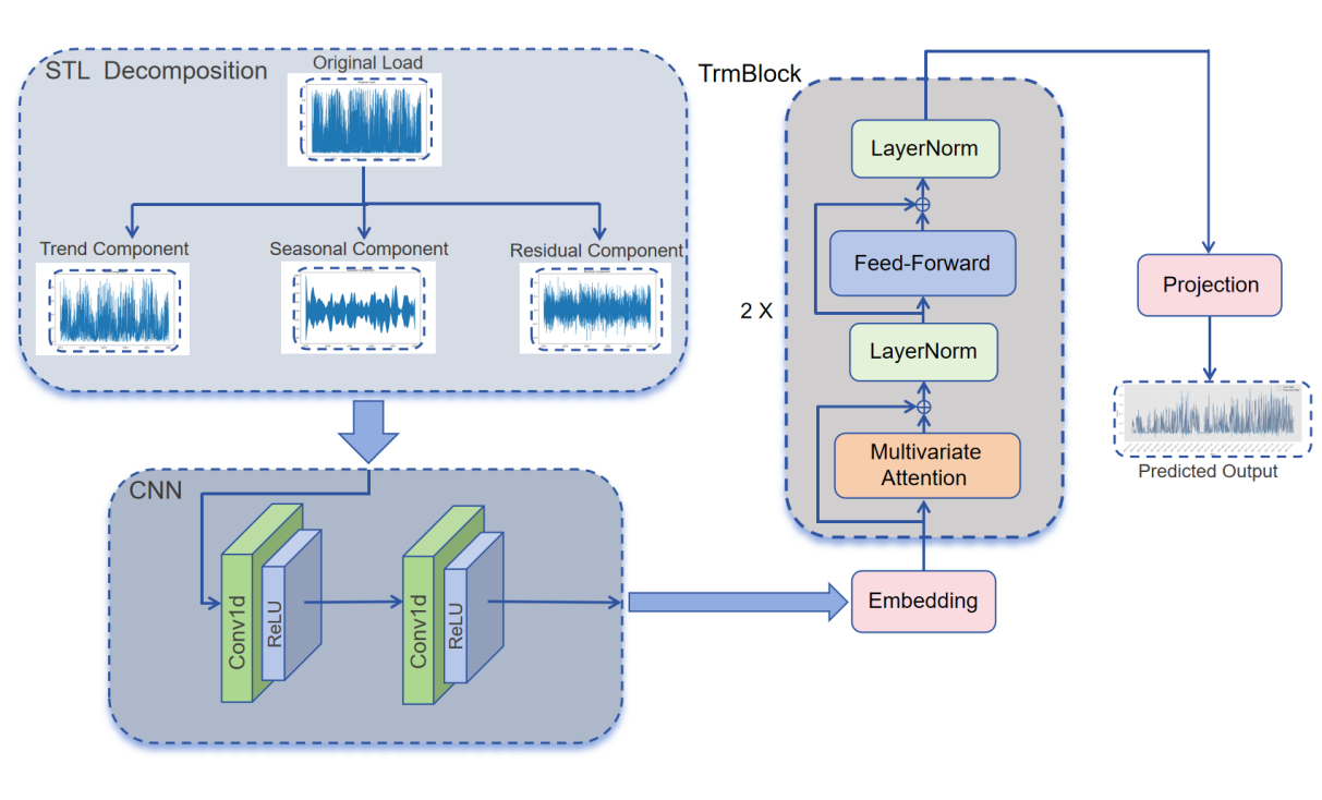
Figure 1: The overall architecture of Sci transformer

3.1. STL

STL (Seasonal-Trend decomposition using Loess) is a time series decomposition technique based on locally weighted regression (LOESS), with its primary advantages being non-parametric flexibility and robustness. Unlike traditional decomposition methods, such as moving averages, or frequency-domain approaches, such as Fourier Transform or Empirical Mode Decomposition (EMD), STL does not rely on any prior assumptions regarding the forms of trend or seasonal components. Instead, it captures patterns across different scales through LOESS fitting. This characteristic makes STL particularly suitable for complex time series that exhibit non-stationarity, varying amplitudes, or structural shifts, offering strong interpretability and adaptability. STL decomposes the original time series into three main components: Trend, Seasonality, and Residual, as follows:

\( {Y_{v}}={T_{v}}+{S_{v}}+{R_{v}} \)

Where \( {Y_{v}} \) denotes the original observation at time point \( v \) ; \( {T_{v}} \) represents the trend component, reflecting long-term structural changes; \( { S_{v}} \) captures the seasonal component, characterizing periodic fluctuations; and \( {R_{v}} \) corresponds to the remainder component, encompassing local perturbations, anomalous variations, and other non-systematic noise elements.

3.2. CNN

Convolutional Neural Networks (CNNs) were initially widely applied in image recognition and computer vision tasks, with core advantages including local receptive fields, parameter sharing, and hierarchical feature extraction capabilities. With the advancement of deep learning, CNNs have been gradually introduced into time series modeling, demonstrating strong feature extraction and generalization abilities when dealing with structurally complex and highly volatile data. Wind power generation data often contain abrupt changes, disturbances, and short-term fluctuations. Utilizing CNNs enables the effective extraction of local temporal patterns, providing foundational feature representations for further processing by deeper modeling frameworks.

The core components of a CNN include the convolutional layer, activation function, pooling layer, and fully connected layer. In time series modeling, one-dimensional convolution (1D-CNN) is commonly employed to perform sliding window operations along the temporal dimension, enabling the extraction of local features. In 1D convolution, the input sequence \( X=\lbrace {x_{1}},{x_{2}},,{x_{T}}\rbrace \) is convolved with a kernel \( W=\lbrace {w_{1}},,{w_{k}}\rbrace \) through sliding inner products, and the resulting feature map can be expressed as:

\( f(t)=\sum _{i=0}^{k-1}{w_{i}}*{x_{t+i}}+b \)

Where \( k \) denotes the kernel size and \( b \) represents the bias term. By applying multiple convolutional kernels in parallel, CNNs are capable of simultaneously capturing local features at different scales, such as trend inflection points, variations in periodic amplitude, and local anomalies.

3.3. iTransformer

Since its introduction, the Transformer model has demonstrated strong capabilities across various sequence modeling tasks, particularly excelling over traditional recurrent neural networks in capturing long-range dependencies and enabling parallel computation. However, in the field of time series forecasting, especially in multivariate prediction scenarios, the standard Transformer architecture faces structural mismatches with the inherent characteristics of time series data. To address this issue, a structurally innovative model, iTransformer, has been proposed [13], whose core idea is to invert the conventional modeling dimension by treating variables as tokens, thereby reconstructing the application of attention mechanisms in time series modeling.

ITransformer fundamentally reverses the design of the standard Transformer by shifting attention modeling from the temporal dimension to the variable dimension and employing feed-forward networks (FFNs) to model temporal dynamics. This results in a more efficient, decoupled, and adaptable architecture. The iTransformer model mainly consists of three modules: Embedding, TrmBlock, and Temporal Projection.

The model accepts an input multivariate time series with a shape of \( X∈{R^{T×N}} \) , where T denotes the number of time steps and N represents the number of variables. Unlike conventional Transformers that treat each time step as a token, iTransformer treats each variable as an independent token, represented by its full sequence of observations across all time steps. The Embedding layer maps each variable sequence into a unified high-dimensional feature space through linear transformation and dropout operations, thus generating N token embeddings as the foundation for subsequent modeling.

The core modeling component consists of several stacked Transformer encoding blocks (TrmBlocks), each containing two key substructures: Series-wise Attention and Time-wise FFN. Series-wise Attention focuses on modeling dependencies between variables by computing attention weights along the variable dimension, effectively capturing the static or dynamic coupling relationships among physical quantities such as wind speed, wind direction, and temperature. Time-wise FFN, on the other hand, performs feed-forward modeling on the time series of each variable individually to extract trend changes and dynamic features. Additionally, each TrmBlock incorporates residual connections and layer normalization to enhance training stability and representational capacity.

The model output is produced by the Projection layer, which maps the representations from the TrmBlocks into the target forecasting space through a linear transformation. It generates prediction results with a shape of \( \hat{Y}∈{R^{T \prime ×N}} \) , where \( T \prime \) represents the forecasting horizon. This module can flexibly accommodate both multi-step rolling prediction and parallel forecasting settings.

3.4. Discription of datasets

The datasets used in this study were obtained from four wind detection stations available on Kaggle. The time span covers from January 2, 2017, 02:00 to December 21, 2021, 23:00, with data sampled at an hourly frequency. Each dataset thus contains 43,801 records. The detailed descriptions of the dataset variables are provided in Table 1.

Table 1: Variable descriptions

The interval length, time step, and number of variables for each real-world dataset are shown in Table 2:

Table 2: Dataset statistics

3.5. Model parameter settings

In the proposed SCiTransformer model, the STL decomposition employs a seasonal cycle window length of 91, with the trend component smoothed using a LOESS window length of 139. The CNN module consists of two layers of 1D convolution, with channel dimensions set to [9, 64] and [64, 64], respectively, and a kernel size of 3. The iTransformer module adopts a two-layer encoder structure, with 8 attention heads, an embedding dimension of 64, a feed-forward dimension of 256, and a dropout rate of 0.1. The entire model is trained using the Adam optimizer, with an initial learning rate of 0.001, a batch size of 64, and a maximum of 50 training epochs.

3.6. Evaluation metrics

To comprehensively evaluate the performance of the wind power forecasting models, this study adopts the Mean Squared Error (MSE) and Mean Absolute Error (MAE) as the primary evaluation metrics. These two metrics characterize the model’s prediction error from different perspectives and effectively reflect its accuracy and stability.

(1) MAE: MAE measures the average absolute deviation between the predicted values and the true values, reflecting the overall “magnitude” of prediction errors with strong interpretability. MAE assigns equal weight to the errors of all sample points and is relatively insensitive to outliers. Its calculation formula is given by:

\( MAE=\frac{1}{n}\sum _{i=1}^{n}|{\hat{y}_{i}}-{y_{i}}| \)

Where \( n \) denotes the number of samples, \( {y_{i}} \) represents the actual value, and \( {\hat{y}_{i}} \) denotes the predicted value by the model.

(2) MSE: MSE measures the mean of the squared prediction errors and is commonly used to assess the overall deviation of predicted values from actual values. Compared to MAE, MSE is more sensitive to larger errors due to the squaring operation, imposing a greater penalty on outliers. Its calculation formula is given by:

\( MSE=\frac{1}{n}\sum _{i=1}^{n}({\hat{y}_{i}}-{y_{i}}{)^{2}} \)

4. Results

In the comparative experiments presented in this study, the primary objective is to validate and demonstrate the effectiveness and superiority of the proposed SCiTransformer model through performance comparisons with seven mainstream time series forecasting methods. By utilizing MSE and MAE as the main evaluation metrics across four datasets from different locations, the experiments in this section not only illustrate the prediction accuracy of each model on specific datasets but also highlight the strong capability of the SCiTransformer model in handling complex data scenarios.

4.1. Comparison of experimental results

To further validate the effectiveness of the proposed SCiTransformer model in practical wind power forecasting tasks, experiments were conducted on four representative wind farm datasets. The predicted results and the corresponding ground truth values for each dataset are visualized in Figure 2. The figure illustrates the model’s fitting capability and trend-capturing performance across different time periods, providing a visual evaluation of its forecasting performance under multi-period and multi-disturbance conditions. From the comparisons, it can be observed that the SCiTransformer model consistently tracks the variations in the ground truth curves across all four datasets, demonstrating strong modeling capabilities in capturing trend fluctuations, local perturbations, and overall structural patterns.

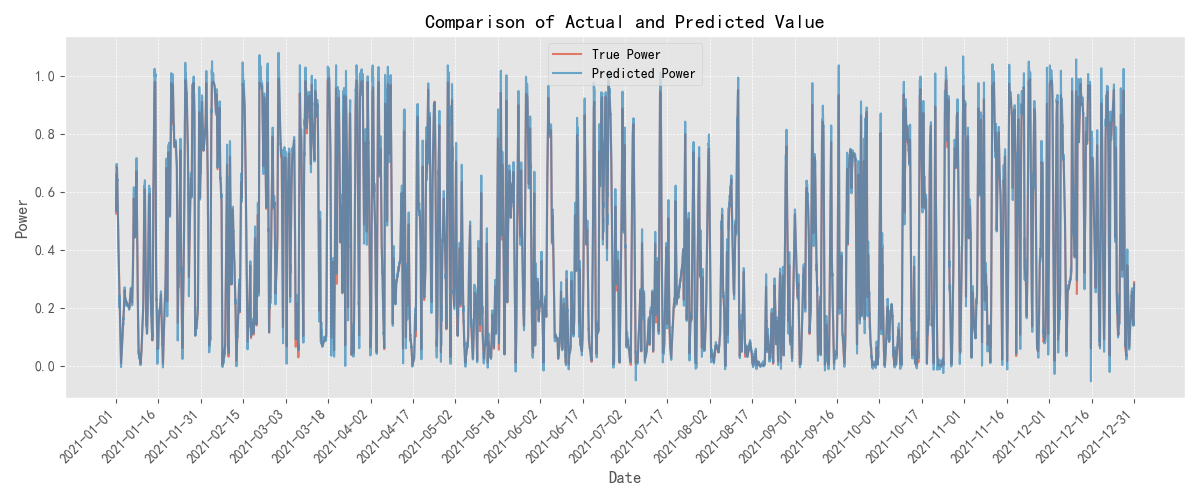
Figure 2(a): Comparison between the ground truth and predicted values at location 1

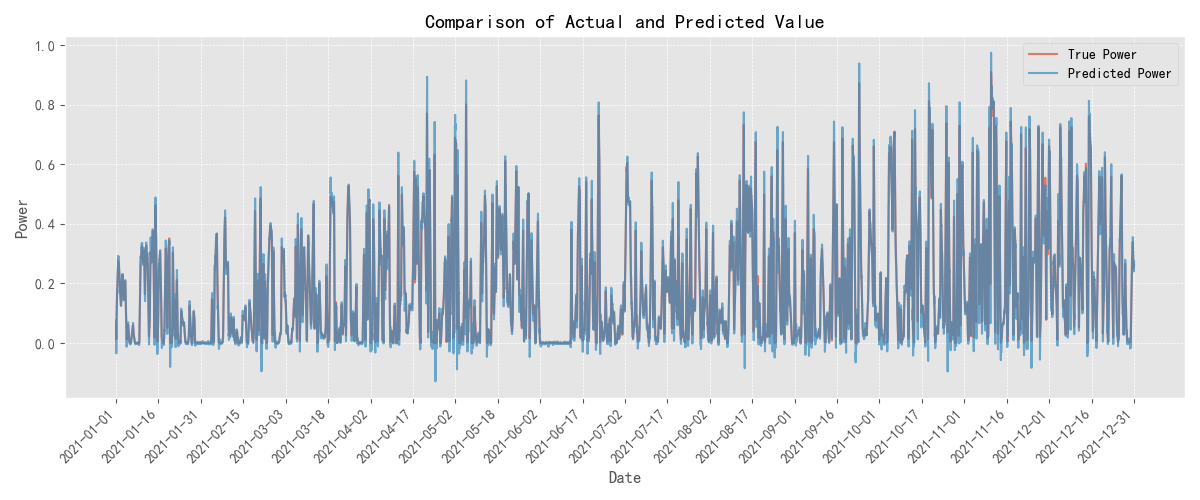
Figure 2(b): Comparison between the ground truth and predicted values at location 2

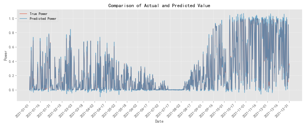
Figure 2(c): Comparison between the ground truth and predicted values at location 3

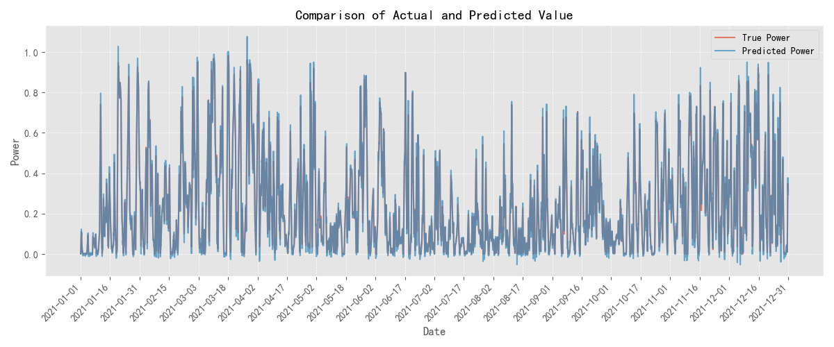
Figure 2(d): Comparison between the ground truth and predicted values at location 4

This study compares the SCiTransformer model with eight different time series forecasting methods, evaluating their performance on datasets from four locations. The evaluation is based on two metrics: MAE and MSE. The experimental results are summarized in Table 3.

Table 3: Comparison of different forecasting methods on location 1, 2, 3 and 4

Note: Red indicates the best performance, and blue indicates the second-best performance.

From the overall results, DLinear achieves the best MSE performance across all datasets. Specifically, the MSE values on Location 1, Location 2, Location 3, and Location 4 are 0.001745, 0.001314, 0.001723, and 0.001154, respectively, all of which are the lowest among the compared models. This suggests that the linear decomposition-based forecasting strategy exhibits strong adaptability when modeling the trend components in wind power data. However, in terms of MAE, DLinear does not consistently outperform other models. For instance, on Location 2 and Location 4, the SCiTransformer achieves MAE values of 0.020473 and 0.020537, respectively, which are 24.6% and 20.3% lower than those of DLinear. This indicates that SCiTransformer offers advantages in controlling stepwise prediction errors, particularly in multi-step rolling forecasting scenarios where error accumulation needs to be mitigated.

Among the other models, Informer and iTransformer demonstrate moderate overall performance. On Location 3, Informer achieves an MAE of 0.059952, slightly better than iTransformer (0.063745) and TimesNet (0.064694). Although iTransformer, with its “variable-as-token” modeling strategy, shows certain advantages in multivariate forecasting, it lags slightly behind in terms of stability and error control. FEDformer and Non-stationary Transformer exhibit relatively higher errors. For instance, FEDformer reaches an MSE of 0.017418 on Location 1, which is approximately ten times that of DLinear, indicating that its frequency-domain enhancement mechanism is less effective for highly non-stationary wind power data. Non-stationary Transformer records the highest MAE across all models, reaching 0.122805 on Location 1, suggesting that its structural design still needs improvement to better adapt to real-world wind power forecasting scenarios. TimesNet shows relatively stable performance, maintaining MAE values around 0.060 across the four datasets. Although it avoids extreme high errors, it does not exhibit significant advantages either. As a structure based on two-dimensional temporal feature modeling, TimesNet has certain strengths in multi-scale trend modeling but remains limited in handling local perturbations.

From a single dataset perspective, Location 2 exhibits the lowest errors among all sites, with most models achieving relatively low MSE and MAE values, possibly due to more regular wind speed patterns at this site. In contrast, Locations 1 and 3 show generally higher error levels and more significant differences among models. For example, Non-stationary Transformer records an MAE of 0.122805 on Location 1, while SCiTransformer achieves only 0.052935 on the same dataset, representing more than a twofold difference.

Overall, SCiTransformer demonstrates outstanding MAE control, particularly under complex disturbance and multi-period conditions, consistently maintaining stable forecasting performance across multiple datasets. Its structural design achieves a well-coordinated layered modeling of trends, periodicities, and disturbances, providing a more robust and reliable solution for wind power forecasting tasks.

4.2. Ablation study

To further verify the effectiveness of the STL decomposition module and the CNN module within the overall model, two groups of ablation experiments were designed to compare the performance of the complete SCiTransformer model with its two variant structures. The first variant, STL-iTransformer, removes the CNN module and relies solely on the iTransformer for global modeling. The second variant, CNN-iTransformer, removes the STL decomposition and directly models the raw wind power sequences. Experimental results show that removing either of these key modules leads to a significant decline in prediction accuracy, indicating that both modules play indispensable roles within the overall architecture. The comparison of MSE and MAE metrics for the three models across the four wind farm datasets is illustrated in Figure 3.

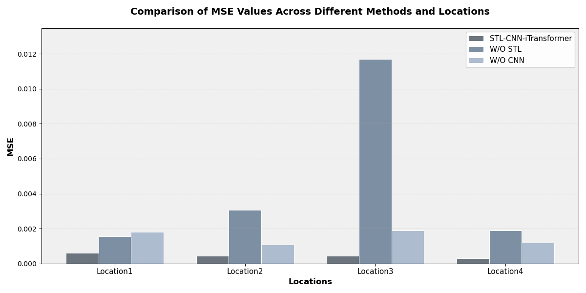
Figure 3(a): Comparison of MSE values across different methods and locations

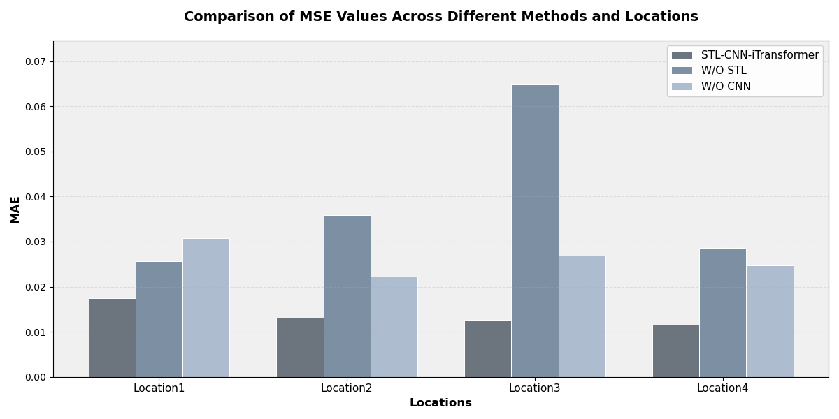
Figure 3(b): Comparison of MAE values across different methods and locations

From the results, the complete model (SCiTransformer) consistently outperforms the two ablated variants in terms of both MSE and MAE across all datasets. For instance, on Location 3, the MSE of the proposed model (“Ours”) is 0.000439, representing a reduction of 96.2% compared to “CNN+iTransformer” (0.011707) and 76.6% compared to “STL+iTransformer” (0.001880). Similarly, in terms of MAE, the proposed model achieves an 80.6% and 53.1% reduction compared to the two variants, respectively. This performance gap is consistently observed across the other three datasets as well, indicating that both the STL decomposition and the CNN modules play critical roles in enhancing the forecasting accuracy of the overall model.

Specifically, after removing the STL module, the model exhibits a substantial increase in errors across multiple sites, indicating that time series decomposition is critical for capturing the trend and periodic structures inherent in wind power sequences. Conversely, when the CNN module is removed, the model still maintains a certain level of accuracy but shows noticeably weaker performance in responding to local perturbations and abrupt changes, highlighting the important role of CNN in residual modeling.

The experimental results validate the complementary roles of the STL and CNN modules: the former is responsible for structural decomposition, while the latter enhances local pattern perception. Their collaboration significantly improves the representational capacity and generalization performance of the iTransformer backbone.

5. Conclusion

This study addresses the challenges of non-stationarity, multi-periodicity, and disturbance uncertainty widely present in wind power forecasting tasks, and proposes a deep learning framework—SCiTransformer—that integrates time series decomposition, local modeling, and global attention mechanisms. The model explicitly extracts trend, seasonal, and residual structures through the STL decomposition module, focuses on short-term perturbations with the CNN module, and captures global dependencies among variables using the iTransformer, thus achieving a coordinated unification of structural decomposition and feature modeling. Empirical results on four real-world wind farm datasets demonstrate that the proposed model significantly outperforms mainstream baseline models in terms of MSE and MAE, showcasing superior forecasting accuracy, cross-scenario robustness, and multi-scale modeling capability. Compared with single-path deep learning models, SCiTransformer emphasizes structured feature separation and hierarchical representation, exhibiting strong adaptability in modeling complex periodic disturbances, enhanced variable couplings, and extreme weather conditions. The ablation studies further confirm the critical roles of the STL and CNN modules, indicating that the model not only has a structurally sound design but also effectively achieves multi-source information integration at the mechanism level. Importantly, this study not only improves the numerical accuracy of forecasting results but also provides more interpretable and practical technical support for wind farm scheduling, power system optimization, and renewable energy integration.

The proposed SCiTransformer not only provides a high-performance solution for wind power forecasting but also represents a systematic modeling paradigm based on “data decomposition—feature modeling—information integration.” Future research could further incorporate multimodal meteorological data, graph-structured modeling methods, and transfer learning strategies to expand the input dimensions, structural generalization, and application adaptability of the model. Moreover, exploring its deployment potential in regional wind power optimization, intelligent grid management, and other real-world energy scenarios would be a valuable direction for future work.

References

[1]. Sapankevych, N. I., and Sankar, R. (2009). Time series prediction using support vector machines: A survey. IEEE Computational Intelligence Magazine, 4(2), 24–38.
[2]. Tay, F. E. H., and Cao, L. (2001). Application of support vector machines in financial time series forecasting. Omega, 29(4), 309–317.
[3]. Kane, M. J., Price, N., Scotch, M., and Rabinowitz, P. (2014). Comparison of ARIMA and Random Forest time series models for prediction of avian influenza H5N1 outbreaks. BMC Bioinformatics, 15(1), 1–9.
[4]. Drisya, G. V., Asokan, K., and Kumar, K. S. (2022). Wind speed forecast using random forest learning method. arXiv preprint, arXiv:2203.14909.
[5]. Nakagawa, K., and Yoshida, K. (2022). Time-series gradient boosting tree for stock price prediction. International Journal of Data Mining, Modelling and Management, 14(2), 110–125.
[6]. Xie, A., Yang, H., Chen, J., Sheng, L., and Zhang, Q. (2021). A short-term wind speed forecasting model based on a multi-variable long short-term memory network. Atmosphere, 12(5), 651.
[7]. Lai, G., Chang, W.-C., Yang, Y., and Liu, H. (2018). Modeling long- and short-term temporal patterns with deep neural networks. ACM SIGIR Conference on Research and Development in Information Retrieval, 41(1), 95–104.
[8]. Zhou, H., Zhang, S., Peng, J., Zhang, S., Li, J., Xiong, H., and Zhang, W. (2021). Informer: Beyond efficient transformer for long sequence time-series forecasting. Proceedings of the AAAI Conference on Artificial Intelligence, 35(12), 11106–11115.
[9]. Wu, H., Xu, J., Wang, J., and Long, M. (2021). Autoformer: Decomposition transformers with auto-correlation for long-term series forecasting. Advances in Neural Information Processing Systems, 34, 22419–22430.
[10]. Hao, J., & Liu, F. (2024). Improving long-term multivariate time series forecasting with a seasonal-trend decomposition-based 2-dimensional temporal convolution dense network. Scientific Reports, 14(1), 1689.
[11]. Lim, S., Park, J., Kim, S., Wi, H., Lim, H., Jeon, J., Choi, J., and Park, N. (2023). Long-term time series forecasting based on decomposition and neural ordinary differential equations. Proceedings of the 2023 IEEE International Conference on Big Data (BigData), 748–757.
[12]. Cao, H., Huang, Z., Yao, T., Wang, J., He, H., and Wang, Y. (2023). InParformer: Evolutionary decomposition transformers with interactive parallel attention for long-term time series forecasting. Proceedings of the AAAI Conference on Artificial Intelligence, 37(6), 6906–6915.
[13]. Liu, Y., Hu, T., Zhang, H., Wu, H., Wang, S., Ma, L., and Long, M. (2023). iTransformer: Inverted transformers are effective for time series forecasting. arXiv preprint arXiv:2310.06625.
Cite this article
Jiang,Y.;Cheng,Y. (2025). SCiTransformer: A Trend-Decomposition-Guided Spatio-Temporal Convolution Enhanced iTransformer for Wind Power Forecasting. Applied and Computational Engineering,162,93-104.
Data availability
The datasets used and/or analyzed during the current study will be available from the authors upon reasonable request.
Disclaimer/Publisher's Note
The statements, opinions and data contained in all publications are solely those of the individual author(s) and contributor(s) and not of EWA Publishing and/or the editor(s). EWA Publishing and/or the editor(s) disclaim responsibility for any injury to people or property resulting from any ideas, methods, instructions or products referred to in the content.
About volume
Volume title: Proceedings of CONF-FMCE 2025 Symposium: Semantic Communication for Media Compression and Transmission
© 2024 by the author(s). Licensee EWA Publishing, Oxford, UK. This article is an open access article distributed under the terms and
conditions of the Creative Commons Attribution (CC BY) license. Authors who
publish this series agree to the following terms:
1. Authors retain copyright and grant the series right of first publication with the work simultaneously licensed under a Creative Commons
Attribution License that allows others to share the work with an acknowledgment of the work's authorship and initial publication in this
series.
2. Authors are able to enter into separate, additional contractual arrangements for the non-exclusive distribution of the series's published
version of the work (e.g., post it to an institutional repository or publish it in a book), with an acknowledgment of its initial
publication in this series.
3. Authors are permitted and encouraged to post their work online (e.g., in institutional repositories or on their website) prior to and
during the submission process, as it can lead to productive exchanges, as well as earlier and greater citation of published work (See
Open access policy for details).