1. Introduction

Road sign recognition technology refers to the use of computer vision technology to identify, detect and analyze road signs in images. It is also known as Traffic-sign recognition (TSR), is a technology by which a vehicle is able to recognize traffic signs on the road such as "speed limit" or "children" or "turn ahead" [1]. As an important technology in autonomous driving tasks, road sign recognition technology perceives road environment information to provide a key decision-making basis for vehicle driving, which can improve the safety and stability of autonomous vehicles. In recent years, with the rapid development of intelligent transportation and autonomous vehicles, road recognition technology has attracted a lot of research interest from academia and industry, which has been widely used in many derivatives tasks, such as geographic information systems, indoor positioning systems, and vehicle management system.

Road sign recognition technology was developed in the early 1980s and has been taken a great step in the field of autonomous vehicles in 1987 [2]. Most of the early traffic road recognition methods are based on manual features, such as using color, texture, contour, shape and other features. Common ones are those based on the shape of the sign board. Typical sign board shapes like hexagons, circles, and rectangles define different types of signs, which can be used for classification [3]. Common methods mainly include color enhancement, color clustering, color segmentation, image matching, feature extraction, digital morphology, set transformation, geometric reasoning, and color space thresholding. Although the above methods have made some progress in the field of automatic traffic sign recognition, the recognition accuracy is still difficult to meet the stringent requirements of practical applications, and the method design needs to rely on prior knowledge, which cannot make full use of the advantages of big data. Modern traffic-sign recognition systems are being developed using convolutional neural networks, mainly driven by the requirements of autonomous vehicles and self-driving cars [4], and the performance of some excellent convolutional neural network models on image recognition tasks has surpassed that of traditional manual feature recognition methods. Therefore, researchers began to seek ways to improve the accuracy of automatic traffic sign recognition through deep learning technology. In 2018, a CNN-based approach to road sign recognition achieved 99.46% accuracy on the German traffic sign dataset. In 2019, researchers achieved over 99% accuracy on a dataset of US road signs using a CNN-based approach. In 2020, the CNN-based road sign recognition method achieved an accuracy rate of 98.71% on the Chinese city road sign dataset [5].

Focusing on the above aspects, we will review the basic theories of the three representative methods in detail in Section 2, and introduce the details of the original dataset and model construction in Section 3. In Section 4, we report the results of different methods. Finally, we summarize the possible problems of traffic sign recognition and look forward to its future development.

2. Revisit basic theory

2.1. Support vector machine (SVM)

A support vector machine (SVM) is a machine learning algorithm that uses supervised learning models to solve complex classification, regression, and outlier detection problems by performing optimal data transformations that determine boundaries between data points based on predefined classes, labels, or outputs [6]. It is a powerful and versatile algorithm that has been used in a variety of applications including text classification, image recognition, and bioinformatics. The main principle behind SVM is to find the hyperplane that best separates the data into two classes. The hyperplane is defined as the line or plane that separates the data points of one class from another. SVM finds the hyperplane by maximizing the margin between the two classes. This is done by finding the point of maximum separation (the Support Vector) and then finding the hyperplane that passes through this point and maximizes the margin between the two classes.

The Support Vector is the point of maximum separation between the two classes. The hyperplane that passes through the Support Vector separates the two classes. This hyperplane can be used to classify new data points. If the data point lies on one side of the hyperplane, it is classified as belonging to one class, and if it lies on the other side, it is classified as belonging to the other class. SVM can also be used for regression problems. In this case, the aim is to find the best fit line that passes through the data points. The SVM algorithm finds the line that minimizes the error between the data points and the line.

2.2. Logistic regression

Logistic regression is a classification algorithm in supervised machine learning algorithm. Usually, the known characteristic variables are used to predict the value of a discrete target variable (such as 0/1, yes/no, true/false). The result variable value obtained by logistic regression fitting is a probability value (0-100%), which is mapped to the classification value of the final prediction target variable according to the size of the probability value and the classification threshold determined according to the business scenario, for example, if the probability value is greater than or equal to 50%, the classification value of the mapping target variable is 1; The probability value is less than 50%, and the classification value of the mapping target variable is 0 [7].

The basic idea of logistic regression is similar to the linear regression. Linear regression is to use the linear combination of features to fit the distribution and trajectory of points in multi-dimensional space for the sample points existing in multi-dimensional space, as the formula (1) shown:

(1)

The formula of is logistic regression as follows:

(2)

where is called sigmoid function. If the classification threshold is 0.5, when h_θ(x)<0.5, then the current sample data is divided into Class A. However, if h_θ(x)>0.5, then divide the current sample data into category B. In conclusion, the sigmoid function can be regarded as the probability function of the sample data.

2.3. Multilayer perceptron (MLP)

The Multilayer Perceptron (MLP) was proposed in 1970 by Rumelhart, Hinton and Williams, which is a typical feedforward neural network consisting of a finite number of successive layers. As shown in Figure 1, each layer consists of a finite number of units (often called neurons). Each unit of each layer is connected to each unit of the subsequent (and thus previous) layer. These connections are generally called links or synapses. Information shows from one layer to the subsequent layer [8]. The model consists of input layer(input), hidden layer (intermediate layer) and output layer(output) [9].

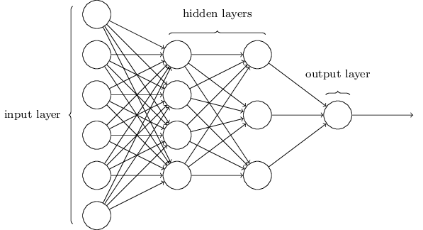
The training process of multilayer perceptron is realized by BP (Back Propagation) algorithm. The main steps are: (1) Set the parameters of the model according to the training set, calculate forward and get the results from the input layer to the output layer. (2) Calculate the loss function and update the parameter model according to the gradient descent algorithm. (3) Do again the forward propagation, until the model training accuracy meets the standards (the model converges). There are three essential factors in the MLP model: Weight, Bias, and Activation function [10], which can be defined as:

(3)

Where represents each neuron, and is weight of each neuron describing the strength of the connections between neurons. is to classify samples correctly and make sure that the output value calculated by the input cannot be activated casually.

3. Model construction

3.1. Original dataset

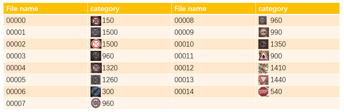
The entire dataset consists of 15 categories of road signs. The specific categories and the amount are as follows in Figure 2. There are 15540 ppm figures in all. Different factors are also considered in the dataset, including gray scale, luminance, definition. The whole 15400 figures are divided into 300 testing set and the rest are training set. The testing set includes 150 figures without noise (clear, full illumination, good weather condition, entitled Testing Set I ), 150 figures of inadequate illumination and good definition (entitled Testing Set II ), 150 figures of adequate illumination but lack of definition (entitled Testing Set III ).

3.2. Model construction of logistic regression

3.2.1. Image preprocessing. The image preprocessing part is used to preprocess the input image for training or testing the deep learning model. For example, when training a convolutional neural network, preprocessing the input image data into a standard normalized form can improve the training speed and accuracy of the model. We first use a torchvision.transforms module to define an image preprocessing sequence of operations. It consists of two steps: (1) Convert the input image data to the torch.tensor format, that is, normalize the pixel values to [0,1]. (2) Normalize the image so that the pixel value conforms to the mean value [0.3659, 0.3103.0.3146], and the standard deviation is [0.2776, 0.2580, 0.2599], and use im_aug to save the image normalization result, as shown in the figure above shown. This normalization can usually improve the training effect of deep learning.

3.2.2. Grayscale processing. We implemented a function weight_gray that converts a color image into a grayscale image, as shown in the figure above. This function can convert a color image into a gray image, which can increase the accuracy of the test. The specific implementation process is as follows: (1) Define three weight coefficients, namely wr, wg, and wb, which represent the weight of converting red, green, and blue channels into gray channels. (2) Create a random tensor grayImg of shape (1,32,32) for storing the converted grayscale image. (3) Calculate the grayscale value of each pixel and set it as the value at the corresponding position of the grayImg tensor. Specifically, for the pixel in the i row and column j, the gray value is wr*Img[0,i,j]+wg*Img[1,i,j]+wb*Img[2,i,j], and then Then divide by 3 to get the pixel value of the grayscale image at the corresponding position. (4) Return the converted image grayImg. The weight_gray function can convert the input color image to a grayscale image. The values of the three weight coefficients wr, wg, and wb can be adjusted as needed to obtain different grayscale images.

3.2.3. Digitization of images. After completing the above work, the author uses the code in the above figure to digitize the image, where trainImages and trainLabels save the images and labels of the image respectively. Specifically, the image data can be reduced in dimension with the flatten function, and flattened into a one-dimensional vector, and the label is converted into an integer type, and stored in the X and Y data respectively to prepare for the training of the subsequent model. It can be understood as converting raw data into a format that can be input into a machine learning model.

3.2.4. Optimal parameter combination. In order to find the best combination of parameters to improve the performance of the model. The author used the logistic regression model to wake up the parameter network search, and the specific code is shown in the figure above. The specific implementation process is as follows:

(1) A parameter grid p_grid is defined, including possible values of three parameters C, fit_intercept and solver. Among them, C represents the regularization parameter, fit_intercept represents whether to fit the intercept, and solver represents the choice of the optimization algorithm.

(2) A LogisticRegression object log is created. The parameter penalty of this object is specified as l2, tol is 0.01, multi_class is 'multinomial', and random_state is 0. Indicates that L2 regularization is performed on the data, the tolerance (tol) is 0.01, the multi-classification method is 'multinomial', and the random seed is 0.

(3) A KFold object cv is created, and the data set (train_X, train_Y) is divided into 5 subsets for cross-validation.

(4) Finally, a GridSearchCV object clf is created, using the parameter grid p_grid defined above, the LogisticRegression object log and the KFold object cv to perform a grid search, find the best parameter combination, and return the best score under this parameter combination. The best score is calculated based on the average cross-validation score, which reflects the performance of the model on the given dataset.

3.2.5. Feature dimensionality reduction based on PCA. We then use the PCA algorithm to reduce the dimensionality of the eigenvalues, the specific code is as above. This function is used to reduce high-dimensional data to low-dimensional data, which can improve the accuracy of the test. The specific functions are as follows:

(1) Transpose the data set X into n d-dimensional samples, where d represents the feature dimension of each sample, and n represents the number of samples. (2) Calculate the mean of each dimension, and subtract the corresponding mean from each dimension of each sample, so that the mean of the data set is 0. (3) Calculate the covariance matrix between different dimensions, where C[i][j] represents the covariance between the i dimension and the j dimension. (4) Perform eigenvalue decomposition on the covariance matrix to obtain eigenvalues and eigenvectors. (5) According to the sorting of the eigenvalues from large to small, the eigenvectors corresponding to the first k eigenvalues are selected as the principal components, and the original data set is projected onto the principal components to obtain the dimensionally reduced data set low_X. (6) Return the dimensionally reduced data set as a new data set X, and return the feature vector EV_main corresponding to the principal component and the mean value mean_X of each dimension. Finally, call the PCA function to get the result after reduction, and save it in the three parameters of low_X, EV_main, and mean_X.

3.2.6. Model training. After completing the above work, the author implemented a machine learning model loaded in Pickle format, and then used the model to predict the given test data set X and label set Y and calculate the accuracy rate. The specific functions are as follows: (1) The pickle library is imported to serialize and deserialize python objects, so that it is convenient to save and load machine learning models. (2) Specify the name of the model file to be loaded as logregModel.sav, and use the pickle.load method to load it into the loaded_model variable in memory. (3) Only use the loaded model loaded_model to predict the wake-up of the test data set X, and calculate its accuracy. Specifically, the loaded_model.score(X, Y) method returns the accuracy of the model on the test data set. (4) Output the best estimator of the loaded model, such as the parameter settings of the model. (5) Output the accuracy of the model on the test data set. Among them, the f-string of Python3.6 is used to format the output string, where {} represents the variable to be inserted.

3.3. Model construction of multilayer perceptron

3.3.1. Image preprocessing. The Torchvision.transforms module is used to define the image preprocessing sequence of the MLP model. The image data is converted to the torch.tensor format and the pixel value is normalized to [0,1]. Then normalize the picture to make the pixel value conform to [0.3659, 0.3103.0.3146], and the standard deviation is [0.2776, 0.2580, 0.2599], and use im_aug to save the image normalization result.

3.3.2. Grayscale processing. Function Weight_gray implemented that converts a color image into a grayscale image. It converts a color image into a gray image, which can increase the accuracy of the test.

The Weight_gray function can convert the input color image to a grayscale image. The values of the three weight coefficients wr, wg, and wb can be adjusted as needed to obtain different grayscale images.

3.3.3. Fourier high-pass filter. Considering that there is still a small amount of noise in the picture, a conventional method is used to deal with the noise in the picture. In the study, Fourier high-pass filter is utilized. CV2 is used to read the image, and Fourier transform is used for high-pass filtering, and then transfer back to image so as to filter the noise from the image.

3.3.4. Feature dimensionality reduction based on PCA. The PCA algorithm is used to reduce the dimensionality of the eigenvalues. Transpose the data set X into n d-dimensional samples, Calculate the mean of each dimension, and subtract the corresponding mean from each dimension of each sample, so that the mean of the data set is 0. Calculate the covariance matrix between different dimensions. Perform eigenvalue decomposition on the covariance matrix to obtain eigenvalues and eigenvectors. The eigenvectors corresponding to the first k eigenvalues are selected as the principal components according to the sorting of the eigenvalues from large to small.

3.3.5. Parameters setting. It is generally believed that within a certain limit, the larger the number of parameters of neural network, the more accurate the results of neural network. The number of layers of the neural network model represents the complexity of the network. The best results can be achieved when the complexity of neural networks matches the complexity of training data and problems. If the sample data is small or the problem is very simple, it is easy to use a complex neural network with many layers to learn, and the final effect is not good.

Based on the above theories, the initial parameters of the MLP model are set. Set the initial total number of neurons as 100 and the activation function as the common activation function, including Logistic, Tanh, RELU. The parameters of each layer are set as average as possible to test the performance of neural network, including a single hidden layer (100), a double hidden layer (50,50) and a triple hidden layer (33,33,33) to test performance.

3.4. Model construction of Linear SVM

3.4.1. Image preprocessing. The Torchvision.transforms module is used to define the image preprocessing sequence of the MLP model. The image data is converted to the torch.tensor format and the pixel value is normalized to [0,1]. Then normalize the picture to make the pixel value conform to [0.3659, 0.3103.0.3146], and the standard deviation is [0.2776, 0.2580, 0.2599], and use im_aug to save the image normalization result.

3.4.2. Grayscale processing. Function Weight_gray implemented that converts a color image into a grayscale image. It converts a color image into a gray image, which can increase the accuracy of the test.

The Weight_gray function can convert the input color image to a grayscale image. The values of the three weight coefficients wr, wg, and wb can be adjusted as needed to obtain different grayscale images.

3.4.3. Fourier high-pass filter. Considering that there is still a small amount of noise in the picture, a conventional method is used to deal with the noise in the picture. In the study, Fourier high-pass filter is utilized. CV2 is used to read the image, and Fourier transform is used for high-pass filtering, and then transfer back to image so as to filter the noise from the image.

3.4.4. Feature dimensionality reduction based on PCA. The PCA algorithm is used to reduce the dimensionality of the eigenvalues. Transpose the data set X into n d-dimensional samples, Calculate the mean of each dimension, and subtract the corresponding mean from each dimension of each sample, so that the mean of the data set is 0. Calculate the covariance matrix between different dimensions. Perform eigenvalue decomposition on the covariance matrix to obtain eigenvalues and eigenvectors. The eigenvectors corresponding to the first k eigenvalues are selected as the principal components according to the sorting of the eigenvalues from large to small.

3.4.5. Parameters setting. In the SVM classifier, the penalty is set as I2 by SVC standard. Hinge is used as SVM loss. Tol is the Tolerance stop standard, which is set at 0.01. The penalty parameter for an error item entitled C is set at [1,10,100]. A GridSearchCV object clf is created, using the parameter grid p_grid defined above, the SVM object log and the KFold object cv to perform a grid search, find the best parameter combination, and return the best score under this parameter combination. The best score is calculated based on the average cross-validation score, which reflects the performance of the model on the given dataset.

4. Experiments and performance analysis

4.1. Results of logistic regression

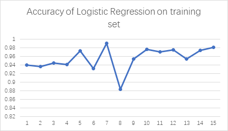
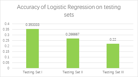
As shown in Figure 3, in the training set, the accuracy of logistic regression is generally lower than that of SVM and MLP models, whose average accuracy is 0.954874. Through image preprocessing of road signs, grayscale processing, image digitization, PCA dimensionality reduction, and test data set, the accuracy rate on the Testing Set I is 0.353333 (53 of 150), which is low compared with MLP and SVM methods. It is due to the influence of parameter processing and the PCA algorithm can only deal with the influence of linear relationship and sensitivity to outliers during grayscale processing. In contrast, the other two methods are better. As shown in Figure 4, according to Testing Set II and Testing Set III, compared with Testing Set I, its accuracy can be lower, whose accuracy is 0.266667 (40 of 150) and 0.22(33 of 150).

4.2. Results of multilayer perceptron

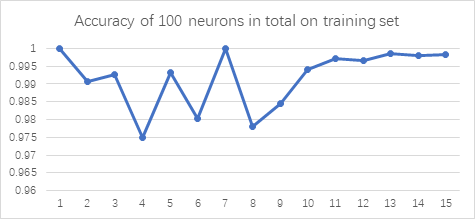
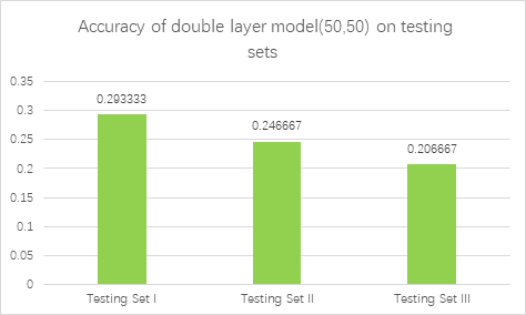
As shown in Figure 4, we first report the accuracy of Multilayer Perceptron on training set and various test sets. When the total number of neurons was 100, the accuracy on training set is above 0.975. The total number of 100 neurons is relatively good for the training set, whose training score can be 0.9911. The best model parameter obtained from Gridsearch is (50,50). But when it turns to the Testing Set I, the accuracy is low, which is 0.293333(44 of 150). The accuracy of Testing Set II and Testing Set III is 0.246667(37 of 150) and 0.206667(31 of 150), which is also low. Note that when the number of parameters is fixed at 100, there is only a high score on the training set, but not a good performance on the test set. This is because the number of neurons is too large, and the sample is overfitted during training, which cannot achieve the desired effect. So the number of parameters is reduced to a total of 60 to prevent overfitting.

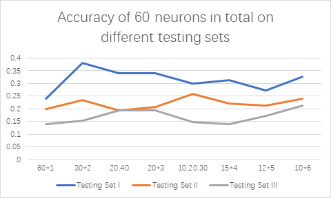
The number of neurons in each layer can also vary, so neuron parameters of one to six different hidden layers are set up for in-depth testing. For 60 neurons, a total of eight different schemes were set up for testing to obtain the optimal scheme, including a single layer (60); 2 double hidden layers (30,30) and (20,40); 2 triple hidden layers (20,20,20) and (10,20,30); 1 four-layer hidden layer (15,15,15,15); 1 five-layer hidden layer (12,12,12,12,12) and 1 six-layer hidden layer (10,10,10,10,10,10). As shown in Figure 5, the total number of 60 neurons is also relatively good for the training set, whose training score can be 0.9864, slightly below the training score of 100 neurons. It’s accuracy of testing set is as follows. It can be found that group (30,30) has the highest accuracy of 0.38 (57 of 150).

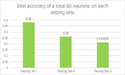
The accuracy of MLP was generally higher than that of Logistic Regression and SVM. For the training set, the accuracy of the MLP model is higher than that of the other two models, with an average accuracy of 0.991764. For the testing set, the accuracy of MLP model on the test set is still not high. For the model group based on the total number of 100 neurons, the best classifier given by gridsearch is (50,50), whose average accuracy on three testing sets is 0.248889. After reducing the total number of neurons to 60, the accuracy of classification models in different groups is tested. For Testing Set I with the least noise, the highest accuracy of the MLP model can reach 0.28, slightly higher than SVM and logistic regression model. Its average accuracy is 0.314167. But accuracy on Testing Set II with low illumination and Testing Set III with low definition is low, whose average accuracy is 0.220833 and 0.169167.

4.3. Results of support vector machine

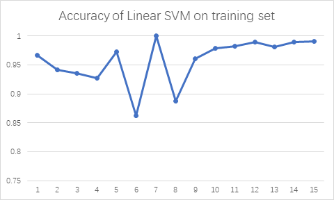
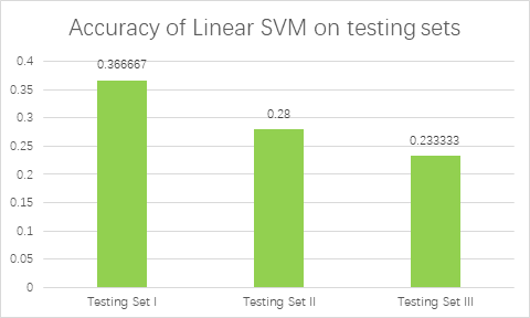
For Linear SVM, as shown in Figure 6, the accuracy of training set is generally higher than that of logistic regression but lower than that of MLP model, whose average accuracy is 0.957889. The accuracy is still low for all three test sets, whose accuracy is 0.366667 (55 of 150), 0.28 (42 of 150) and 0.233333 (35 of 150).

5. Discussion

In this study, we compare the performance of traditional methods such as linear support vector machines, logistic regression, and multilayer perceptrons in the field of road sign recognition with modern methods such as convolutional neural networks. The experimental results show that the accuracy of the traditional method in road sign recognition is relatively low, and there are shortcomings in processing data set format and high-pass filter.

Next, during the data preprocess, we attempted to use filters like bilateral filter, median filter to denoise the image, and method like Canny Edge detection, high pass filter by Fourier Transformation. But all of them, as the images of training dataset is too blurred, or to say, too small in size, the outcome of filter is bad. We visualize the results of Canny Edge detection as an example, which can be see in Figure 7.

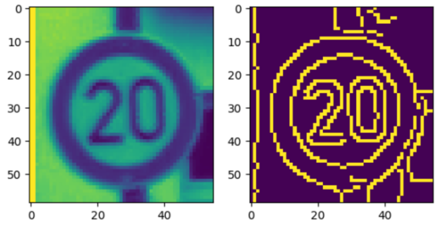
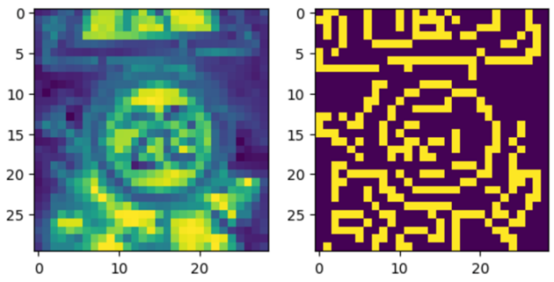
For our training dataset, these methods only performance good on images that clear enough, but bad on images originally blurred which are exactly what needed to be enhanced. As a result, this image preprocess method cannot improve the model, instead, they would decrease the accuracy of model significantly. Also, we found converting the training image into gray image would only decrease the accuracy a little bit but increase the training speed as the number of features decreased.

The significance of this study is that it provides us with an important reference about the limitations of traditional methods in the field of road sign recognition, and shows that modern methods have great advantages in this field. Therefore, we suggest that priority should be given to modern methods in the design and selection of road sign recognition systems to improve traffic safety and efficiency.

6. Discussion

This study mainly discusses the accuracy of traditional linear support vector machine, logistic regression and multi-layer perceptron in the field of road sign recognition, and compares it with the deep learning model (CNN) widely used in modern intelligent vehicles. The effects of illumination and sharpness on these methods were also analyzed. The experimental results show that the accuracy of the three traditional methods is lower than that of CNN, and the accuracy of MLP is the highest, followed by logistic regression, and linear support vector machine is the lowest. The main reason for the low accuracy of traditional methods is that the format of data set we use is not conventional, which is ppm format, and high-pass filter is used, which has poor processing effect on some samples. Under different characteristics of the test set, the accuracy of the three methods is the highest when the light is good and the clarity is good, the accuracy is second when the light is good and the clarity is poor, and the accuracy is the lowest when the light is bad and the clarity is poor. In the training set and the three test sets, the MLP model has the highest comprehensive accuracy, followed by SVM, and the logistic regression has the lowest comprehensive accuracy.

In summary, this study proves that deep learning model has a high accuracy in the field of road sign recognition, while traditional methods such as linear support vector machine, logistic regression and multi-layer perceptron are relatively weak. However, it should be noted that our data set format and high-pass filter and other factors affect the recognition accuracy of traditional methods. In addition, it is found that illumination and sharpness have significant influence on the recognition accuracy. These findings have important implications for improving road sign recognition algorithms and improving the safety of intelligent vehicles.

References

[1]. "What is Traffic Sign Recognition in Cars? - ADAS 101," Oct. 12, 2021. https://caradas.com/understanding-adas-traffic-sign-recognition/.
[2]. J. Xing, M. Nguyen, and W. Yan, "The Improved Framework for Traffic Sign Recognition Using Guided Image Filtering | SpringerLink." https://link.springer.com/article/10.1007/s42979-022-01355-y.
[3]. H. Fleyeh, "(PDF) Traffic and Road Sign Recognition." https://www.researchgate.net/publication/29753563_Traffic_and_Road_Sign_Recognition.
[4]. D. Bradley, "Improving AI road sign recognition." https://techxplore.com/news/2021-07-ai-road-recognition.html.
[5]. N. Youssouf, "Traffic sign classification using CNN and detection using faster-RCNN and YOLOV4," Heliyon, vol. 8, no. 12, p. e11792, Nov. 2022, doi: 10.1016/j.heliyon.2022.e11792.
[6]. V. Kanade, "All You Need to Know About Support Vector Machines." https://www.spiceworks.com/tech/big-data/articles/what-is-support-vector-machine/%20scikit-learn/.
[7]. L. Xiran, L. Yijun, and Z. Sofia, "PAID SEARCH ANALYSIS: CASE OF BIG DATA ANALYTICS FOR FRENCH COSMETIC COMPANY".
[8]. A. Pinkus, "Approximation theory of the MLP model in neural networks," Acta Numer., vol. 8, pp. 143–195, Jan. 1999, doi: 10.1017/S0962492900002919.
[9]. Allan P . Approximation theory of the MLP model in neural networks[J]. Acta Numerica, 1999, 8:143-195.
[10]. S. Bag, "Activation Functions—All You Need To Know!," Analytics Vidhya, Jan. 02, 2023. https://medium.com/analytics-vidhya/activation-functions-all-you-need-to-know-355a850d025e.
Cite this article
Liu,X.;Luo,M.;Xiong,X. (2023). Performance Comparison of Road Sign Recognition Methods based on Machine Learning. Applied and Computational Engineering,8,636-648.
Data availability
The datasets used and/or analyzed during the current study will be available from the authors upon reasonable request.
Disclaimer/Publisher's Note
The statements, opinions and data contained in all publications are solely those of the individual author(s) and contributor(s) and not of EWA Publishing and/or the editor(s). EWA Publishing and/or the editor(s) disclaim responsibility for any injury to people or property resulting from any ideas, methods, instructions or products referred to in the content.
About volume
Volume title: Proceedings of the 2023 International Conference on Software Engineering and Machine Learning
© 2024 by the author(s). Licensee EWA Publishing, Oxford, UK. This article is an open access article distributed under the terms and
conditions of the Creative Commons Attribution (CC BY) license. Authors who
publish this series agree to the following terms:
1. Authors retain copyright and grant the series right of first publication with the work simultaneously licensed under a Creative Commons
Attribution License that allows others to share the work with an acknowledgment of the work's authorship and initial publication in this
series.
2. Authors are able to enter into separate, additional contractual arrangements for the non-exclusive distribution of the series's published
version of the work (e.g., post it to an institutional repository or publish it in a book), with an acknowledgment of its initial
publication in this series.
3. Authors are permitted and encouraged to post their work online (e.g., in institutional repositories or on their website) prior to and
during the submission process, as it can lead to productive exchanges, as well as earlier and greater citation of published work (See
Open access policy for details).