1. Introduction

Multi-armed bandit problems play a simplified setting for reinforcement study, where the environment is composed of a slot machine with k arms, each of which has an unknown reward. The goal is to maximize the reward gained from pulling n rounds. Designing algorithms to solve multi-armed bandit problems is important as a path to solve complex reinforcement learning problems, as it presents a non-associative, evaluative feedback problem that reinforcement learning is aimed to solve [1].

Cumulative regret (R) is defined as the difference between the biggest possible rewards and the actual total rewards of n rounds:

\( R=\sum _{t=1}^{n}({{μ_{t}}^{*}}-{μ_{t}}) \) (1)

As stated previously, those algorithms sought to maximize total reward from n rounds of the game, then it is equivalent to minimize total regret R. To compare if an algorithm performs well in solving multi-armed bandit problems, it is important to present its regret curve and compare with others. In the paper, the Thompson \( ε \) -Greedy (TEG) algorithm will be proposed under the context of stochastic stationary bandit problems, its regret curve will be compared with other popular algorithms, and its advantages and disadvantages will be analyzed for its best practical purposes.

2. Developments

Among different types of multi-armed bandit problems, the stochastic stationary multi-armed bandit is defined as an environment where there is a set of distributions \( v=({P_{a}}:a∈A) \) , with \( A \) being all possible actions [2]. Under the reinforcement learning model where the agent and the environment interact for n rounds of the game, the agent will pick an action \( {A_{t}} \) each round and the environment will then sample from \( {P_{{A_{t}}}} \) distribution and return a reward \( {μ_{t}} \) . The distribution of each possible action is stationary and will change with time. And then the goal is for an agent to use \( {μ_{t}} \) of each round to make better decisions in the future and reduce the total regret \( R \) .

An intuitive policy is to apply the explore-then-commit (ETC) algorithm [3]. In ETC, each arm of the bandit is pulled for the same number of rounds m as an exploration phase, and then in the exploitation phase, the arm with the best mean reward \( {\hat{μ}_{i}} \) from the exploration phase will be pulled for the rest of rounds n - mk. Suppose there are k arms, then the decision of action for the round t is:

\( {A_{t}}=\begin{cases} \begin{array}{c} (t mod k)+1, t≤mk \\ {argmax_{i}} {\hat{μ}_{i}}(mk), otherwise \end{array} \end{cases} \) (2)

A disadvantage of the algorithm is that m is hard to decide. To minimize R, both n and the suboptimality gap (the mean difference between an arm and the best arm) need to be known, or a threshold should be set for the exploration phase as proposed in the paper On Explore-Then-Commit Strategies [4].

Then to deal with the disadvantages provided by ETC, the Upper Confidence Bound (UCB) algorithm was designed [5,6]. Instead of exploring and exploiting separately, an upper bound of UCB index for each arm is created, which takes the number of times an arm is selected into account. Then the next action is always the one with the highest upper bound rewards, so the prior knowledge of suboptimality gaps is no longer essential in deciding the best actions.

In the epsilon-greedy algorithm ( \( ε \) -greedy), a parameter \( ε \) is used as the probability of exploration. Suppose there are k arms, then in each round, a random arm is chosen with \( ε \) probability, and the arm with the best mean so far is chosen with 1- \( ε \) probability:

\( {A_{t}}=\begin{cases} \begin{array}{c} random i∈\lbrace 1, 2,…,k\rbrace , ε \\ {argmax_{i∈\lbrace 1, 2,…,k\rbrace }} {\hat{μ}_{i}}(t-1), 1-ε \end{array} \end{cases} \) (3)

It is an action-value method as it uses the sample average to estimate the value of taking an action. An advantage of \( ε \) -greedy is that it allows every action to be taken an infinite number of times, so it ensures that every arm reward estimate converges to its true reward [1]. However, it has a serious weakness that suboptimal arms will continue to be selected in the long run even though they are already identified as suboptimal.

Thompson sampling, an old algorithm that was created by Thompson in 1933 [7], revealed to perform well lately in solving multi-armed bandit problems. It starts with a prior reward distribution on each of the arms. For each round, it samples from each distribution, picks the arm with the greatest reward sample, and uses the feedback of reward to update the distribution of the arm selected. Compared to the UCB algorithm, Thompson sampling performs better when dealing with long delays, as it “alleviates the influence of delayed feedback by randomizing over actions” [8].

3. Problems of \( ε \) -Greedy and Thompson Sampling

3.1. \( ε \) -Greedy

One notable problem of using \( ε \) -Greedy is to pick an appropriate \( ε \) value. If \( ε \) is too low, the model will fail to explore enough so that the optimal arm is missed for a very long time during which the regret is high in every exploitation, whereas if \( ε \) is too high, the model will explore too much to have enough exploitation or keep the regret small:

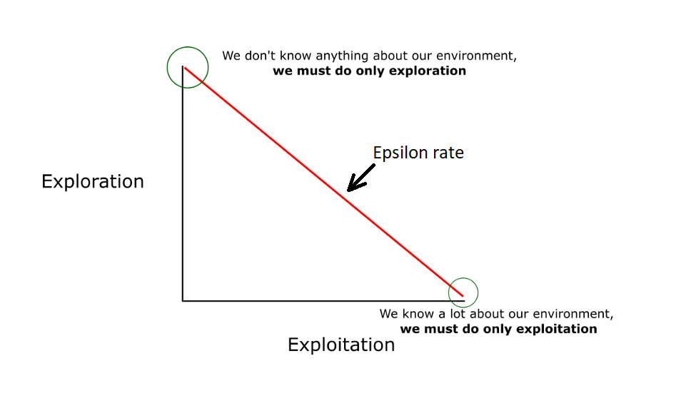
Figure 1. The exploration-exploitation relationship in ε-Greedy (source from PyLessons).

It is noted that even if \( ε \) is tuned to have the optimal fixed value \( {ε^{*}} \) , the regret is still bad because it is linear. Suppose there are k arms, and let \( j∈\lbrace 1, …, k\rbrace \) :

\( E[{R_{t}}]=\sum _{i=1}^{t}[(1-ε)({{μ^{*}}_{i}}-{max_{j}}{({\hat{μ}_{i,j}})})+ε·({{μ^{*}}_{i}}-\frac{\sum _{j}{\hat{μ}_{i,j}}}{k})] \) (4)

As t goes up:

\( E[{R_{t}}]=\sum _{i=1}^{t}ε·({{μ^{*}}_{i}}-\frac{\sum _{j}{μ_{j}}}{k}) \) (5)

So, the regret R is \( Θ(T) \) .

In Finite-time Analysis of the Multiarmed Bandit Problem by Auer et al., making \( ε \) a decreasing function of 1/t successfully turns R to a logarithmic bound [9]. However, \( ε \) -greedy still faces the problem of picking random suboptimal arms, though logarithmic, in the later stage, when it seems to be clear which arm is the best.

3.2. Thompson Sampling

One significant downside of Thompson Sampling is that when two arms have similar regret, it is difficult for it to differ which arm is the best [10]. Suppose there are two arms A, B, with their means \( {μ_{A}} \gt {μ_{B}} \) , and their means are close to each other. If using prior gaussian distribution for Thompson Sampling, at round t, two distributions might look like what is shown in Figure 2:

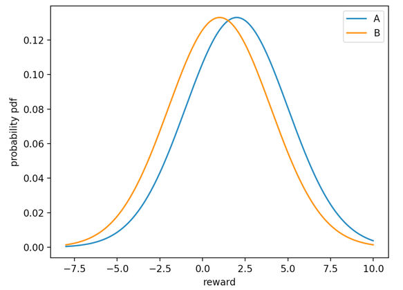
Figure 2. The reward distributions of two arms with a small mean difference.

The probability that a random sample from B is higher than A is significant, so Thompson sampling will frequently pick arm B and increase the regret. Also, if the true reward distributions are scattered, a similar consequence happens as well, due to the high likelihood for a suboptimal arm to have a better sample than the optimal one. In both cases, Thompson sampling will spend a very long time to complete, therefore firms sometimes prefer modifying Thompson sampling to finish it within a reasonable amount of time.

Another disadvantage of Thompson Sampling is that every time an action is chosen, a posterior distribution will be updated to take new reward into account. The process of updating a distribution can be time-consuming. If the multi-armed bandit problem takes n rounds to run and n is very large, the time cost of Thompson Sampling is considerable.

4. Design of Thompson \( ε \) -Greedy Algorithm (TEG)

4.1. Inspiration

In Daniel Russo’s paper Simple Bayesian Algorithms for Best-Arm Identification, he proposed Top-two Thompson Sampling, an algorithm based on Thompson Sampling. Instead of solely picking the arm of the sample with the best reward, Top-two Thompson Sampling has a 1/2 probability to pick the arm with the second-best reward sample [11]. This algorithm improves the rate of the best arm identification at the cost of regret. Though unmatched with the goal of minimizing regret in this paper, his algorithm reminded people that updating the distribution of the best arm with too many rounds will decrease its variance and therefore harm the best identification rate. The reason is intuitive: the distribution of the second-best arm maintains its large variance so there is a high probability that the sample has a reward higher than the best arm sample, as illustrated in Figure 3:

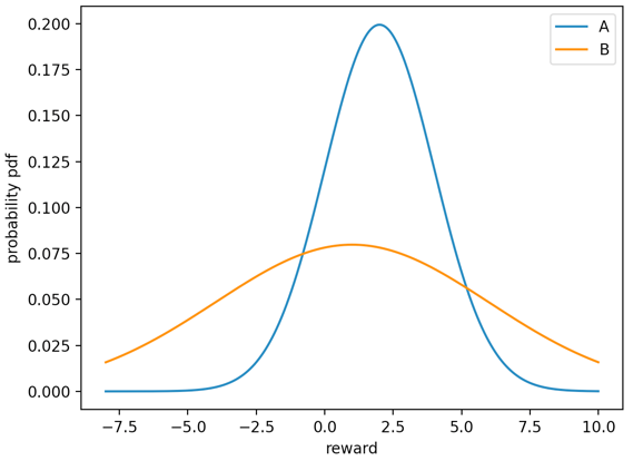
Figure 3. The reward distributions of two arms with significantly different variances.

Perceiving this peculiarity of Thompson Sampling, the author decided to postpone the trend of shrinking the best arm’s distribution, and the solution was to use ε-greedy. It is predicted that implementing Thompson Sampling with ε-greedy could also improve the performance of ε-greedy algorithm’s exploration part, where the exploration would converge to the best arm.

4.2. TEG Algorithm

The design is to use ε-greedy as the framework of the algorithm. In ε-greedy, the arm with the highest mean reward is picked and the mean reward is updated afterwards. Therefore, it is important to record each arm’s mean reward as a global variable. At the same time, to apply Thompson Sampling in the case of exploration, the necessary parameters of reward distributions for each arm are stored. Depending on the prior distribution, different parameters apply, like \( α \) and \( β \) for beta distribution, or mean and variance for gaussian distribution. In the constructor of the algorithm, those variables are declared and initialized.

In the choose function, there are two parts: exploration with a possibility of ε, and exploitation with a possibility of 1-ε. In the exploration stage, the arm with the highest sample reward is chosen, whereas, in the exploitation stage, the arm with the highest mean reward is picked. Note that to improve the performance of the algorithm, each arm is required to be pulled once to rationalize the mean reward and the reward distribution. Besides, the reward distributions are updated only when Thompson Sampling is applied at that round, or otherwise, the best arm’s distribution will shrink too much at the exploitation part to be preferred in the exploration part as previously mentioned. Therefore, a flag representing if it is exploration for this round is returned, so that the update function will be clear on if the reward distribution should be updated.

Lastly, in the update function, the mean reward of the arm that gets picked is updated as its actual reward of the current round is received. Then, check if it is required to update the reward distributions for Thompson Sampling through the Boolean flag that got returned during the choose function. Corresponding to the actual reward of the arm that got picked this round, update the relevant parameters of the reward distribution for the arm if the flag asked for an update (namely, if the flag is true).

4.3. Theoretical feasibility

The author proposes that the TEG algorithm will outperform ε-greedy when using the same ε value. In the exploitation phase, two algorithms do the same process, so the regret difference between the two algorithms depends on the exploration phase and the accuracy of the mean reward.

At each round of the Exploration phase: the expected regret ER for ε-greedy is the average suboptimality gap:

\( {R_{T}}=T\frac{\sum _{i=1}^{K}{Δ_{i}}}{K}=C·T=Θ(T) \) (6)

whereas the expected regret TEGR for TEG in the exploration phase is just the same as Thompson Sampling regret [2]:

\( {TEGR _{T}}=Ο(\sqrt[]{KTlog(T)}) \) (7)

Where T is the number of rounds of exploration, \( {Δ_{i}} \) is the suboptimality gap of arm i, K is the number of arms. As a result, it is guaranteed that \( {TEGR _{T}} \lt {R_{T}} \) when \( Ο(\sqrt[]{KTlog(T)}) \lt Θ(T) \) , i.e., \( K \lt \frac{T}{log⁡(T)} \) . In practice, each arm is always explored at least once for both algorithms, i.e., \( K≤T \) , so it is always that \( K \lt \frac{T}{log⁡(T)} \) . Therefore, it is guaranteed that, in the exploration phase of the TEG algorithm, there is smaller regret than that in the exploration phase of the ε-greedy algorithm, when they use the same ε-greedy value.

Secondly, the author suggests that the accuracy of the mean reward will be more precise for competitive arms and less precise for non-competitive arms. The reason comes from the principle of Thompson Sampling: compared with randomly picking an arm, Thompson Sampling prefers competitive arms to non-competitive arms. As a result, the confidence of competitive arms’ mean rewards is higher in the TEG algorithm than in ε-greedy. In the exploitation phase, competitive suboptimal arms are the main source of the regret, so making competitive arms more precise is a worthy trade-off for making the influential arms’ mean rewards more accurate, increasing the arm identification rate, and decreasing the regret.

Thirdly, it is predicted that the running time for the TEG algorithm will be faster than Thompson Sampling, as the number of times that reward distributions are updated is reduced from 1 to ε each round.

Lastly, the author conjectures that when two arms have similar regret or when true reward distributions are scattered, TEG will have better performance than Thompson Sampling in distinguishing the best reward between arms. Compared to Thompson Sampling which every round compares every arm’s sample from the distribution, TEG spends most of the rounds picking the arm with the best reward mean. The advantage of using the best reward mean instead of the best reward sample is that it ignores the uncertainty of the sample values. While the reward sample’s value could be any point of a distribution’s curve, the mean reward value is fixed at any specific round. The stability of the mean reward gives the author the confidence that it will outperform Thompson Sampling in unfavored environments.

5. Methodology

5.1. Setting

An environment of stochastic stationary bandits is created and the real arm reward distributions are set to a specific kind. Each time an arm is pulled, the real reward returned is a sample of that arm’s reward distribution. Three kinds of distributions are considered: gaussian, Bernoulli, and uniform. Gaussian/Bernoulli represents the cases where the reward could be continuous/binary. The reason for adding uniform reward distribution is to represent the case where the reward is scattered, due to what was previously stated, that Thompson Sampling will not work well in this scenario. Each distribution will create a different experiment to ensure TEG’s generality.

Four arms are created for the bandit, each set with a different true mean reward. When the real reward distribution is gaussian, those four arms’ true means are set to be [5, 7, 9, 11] with a variance of 1. When the real distribution is Bernoulli, true means are set to be [0.05, 0.35, 0.65, 0.95]. When the real distribution is uniform, the true means are set to be [1, 1.7, 2.4, 3.1] each with a range of 1.

5.2. Method

To illustrate the advantage of the TEG algorithm, comparison plots among TEG, ε-greedy, and Thompson Sampling will be drawn, by setting the number of rounds, or the number of trails, to be 3000, and comparing the cumulative regret of all three algorithms. To avoid randomness, 200 independent experiments will be run to calculate the average regret.

5.3. Prior distributions and ε Decision

For TEG and Thompson Sampling, the beta distribution is used as prior when the reward is binary {0, 1}, and the gaussian distribution is used as prior when the reward is continuous. As a result, when the setting reward distribution is Bernoulli, beta is used, whereas when the setting reward is gaussian or uniformed distributed, gaussian prior is used.

To control the variable, both ε-greedy and TEG use the same ε value. From the research result of Auer et al., a recommended decreasing function for ε is a constant term of 1/n, where n is the number of rounds [9]. In practice, tuning the constant factor is difficult, and many would just use 1 as the constant factor. Therefore, \( ε=\frac{1}{n} \) is used as the value for parameter \( ε \) .

6. Experimental result and analysis

6.1. Regret comparison plots

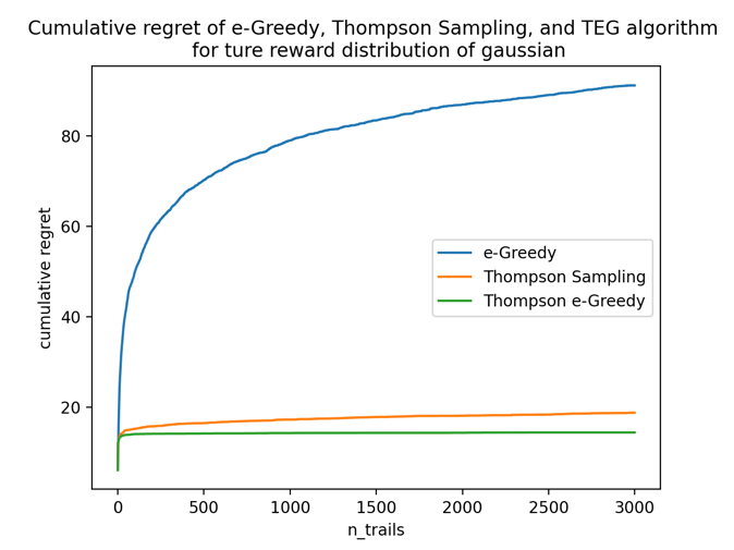
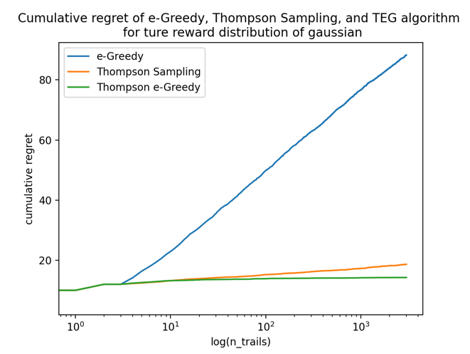
True reward distribution: gaussian.

Prior reward distribution: gaussian.

Figure 4 is the curve of cumulative regret with respect to the number of trails. The blue curve is ε-greedy, the orange one is Thompson Sampling, and the green one is TEG.

Figure 5 is the same curve of the left but scaled the x-axis to logarithmic to prove that the TEG algorithm is also \( Ο(log⁡(N)) \) . Note that here the TEG algorithm outperforms ε-greedy as expected, and it is also slightly better than Thompson Sampling.

True reward distribution: Bernoulli.

Prior reward distribution: beta.

Figure 6 shows that the TEG algorithm outperforms ε-greedy as expected, and slightly loses to Thompson Sampling. the reason behind this is unclear, but one possible explanation is that the prior beta distribution is very sensitive to the change of alpha and beta initially, so it requires a great amount of exploration to make the distribution stable and reasonable, whereas the TEG algorithm fails to explore enough at initially.

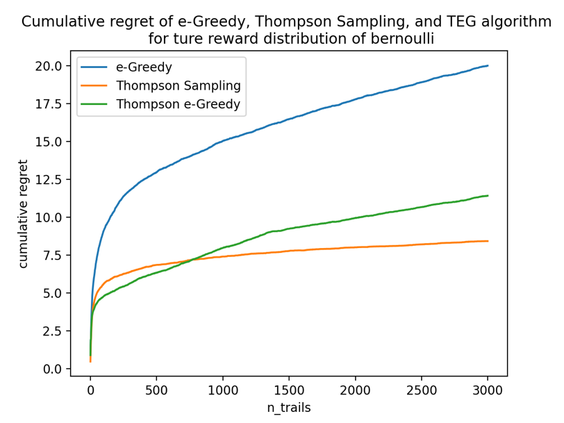
Figure 6. Total regret of three algorithms under bernoulli true rewards.

True reward distribution: uniform.

Prior reward distribution: gaussian.

Figure 7 shows that the TEG algorithm outperforms both ε-greedy and Thompson Sampling as expected. From the graph, the apparent weakened performance of Thompson Sampling matches the author’s analysis of Thompson Sampling’s disadvantage — unfavored scattered distributions. It turns out that the TEG algorithm successfully mitigates the influence of scattered distribution when the reward is continuous.

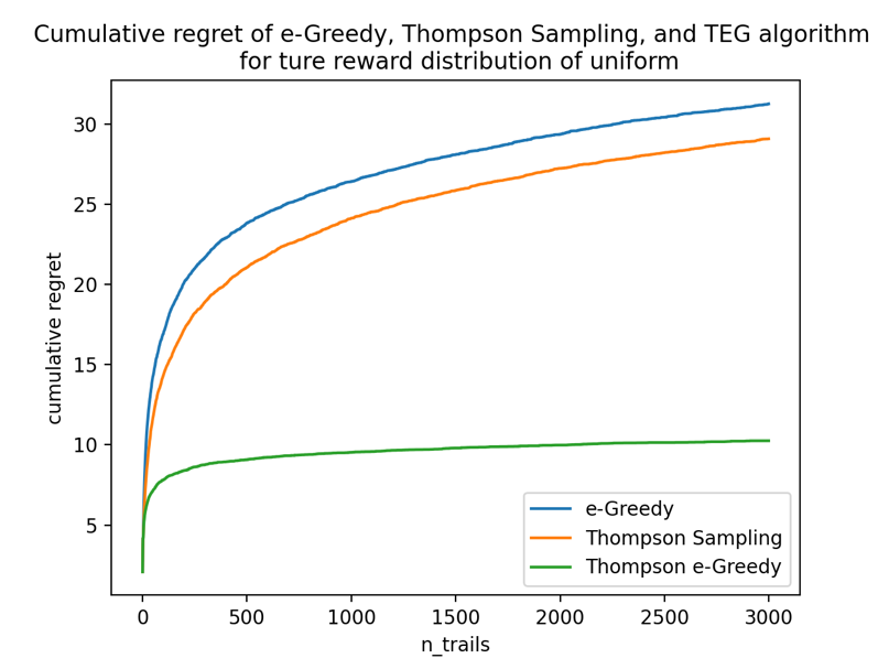
Figure 7. Total regret of three algorithms under uniform true rewards.

6.2. Time comparison table

Besides the regret, a timer is set for each algorithm to compare their running time. The running time in seconds represents the average time to run one experiment for each algorithm in three experiments with different true distributions, as shown in Table 1 below.

Table 1. Average running time of three algorithms on different bandit reward distributions. Running time (sec/exp).

Table 1 shows that the TEG algorithm has a similar time cost as ε-greedy, and runs much faster than Thompson Sampling as expected, suggesting that the TEG algorithm is more time-efficient.

7. Conclusion

From the experiment, the advantages of the TEG algorithm can be summarized as follows: first, the regret of the TEG algorithm is logarithmic in theory and smaller than ε-greedy with the same ε value in general; second, the TEG algorithm is more adaptive to scattered real reward distributions than Thompson Sampling; third, the TEG algorithm has a similar running time to ε-greedy, which is much faster than Thompson Sampling.

Some limitations of the TEG algorithm include: first, when the prior distribution is sensitive to even the smallest unit of change in its parameters, like beta distribution, the TEG algorithm may not reduce the regret as effectively as Thompson Sampling; second, like Thompson Sampling, TEG falls short of recognizing the best arm when the suboptimal arm has very close but a little smaller mean reward.

Due to the significant advantage of the TEG algorithm over ε-greedy, it can replace much work that ε-greedy applies in industries with stochastic multi-armed bandit problems, like clinical tests, advertisements, etc. Since Thompson Sample performed badly in unfavored scattered distributions, like the uniform distribution or U-shape ones, TEG is a good substitution for Thompson Sampling when it is known that the real reward distribution might fluctuate sharply, since TEG has the potential of largely decreasing the regret. Lastly, when a practitioner desires the good performance of Thompson Sampling but struggles against its running time, TEG could be a good solution to the problem.

In this paper, the author designed the TEG algorithm, explored its performance, and explained its advantages. However, several questions remained. The first one is the decision for the ε value. Though \( ε=\frac{1}{n} \) is known as a good value for ε-greedy and TEG outperforms ε-greedy for the same ε value, it does not determine \( \frac{1}{n} \) as the best ε value for TEG. The ε value can be optimized further, and it requires future calculations and experiments. Secondly, the reason for the disadvantage of the TEG algorithm as shown in the first bullet point remains questionable. It is the role of future works to propose and verify the reason behind it. Lastly, the TEG algorithm still fails to cover a disadvantage of Thompson Sampling mentioned in 3.2: the bad performance when two competitive arms have similar mean rewards. That leaves large spaces for further improvements on the TEG algorithm. Future works will aim at a full understanding of the TEG algorithm and optimizing it, making TEG a strong method for multi-armed bandit problems.

Acknowledgements

I would like to appreciate Professor Osman Yagan for supporting the idea and providing relevant documents with guidance to the experiments.

References

[1]. Sutton, R. S. and Barto, A. G. (1998). Reinforcement learning: an introduction. MIT Press.
[2]. Lattimore, T. (2020). Bandit Algorithms. Cambridge University Press. https://doi.org/10.1017/9781108571401.
[3]. Perchet, V., Rigollet, P., Chassang, S. and Snowberg, E. (2016). Batched Bandit Problems. The Annals of Statistics 44(2), 660–681. https://doi.org/10.1214/15-AOS1381.
[4]. Garivier, A., Kaufmann, E. and Lattimore, T. (2016). On Explore-Then-Commit Strategies. https://doi.org/10.48550/arxiv.1605.08988.
[5]. Lai, T. and Robbins, H. (1985). Asymptotically efficient adaptive allocation rules. Advances in Applied Mathematics 6(1), 4–22. https://doi.org/10.1016/0196-8858(85)90002-8.
[6]. Katehakis, M. N. and Robbins, H. (1995). Sequential Choice from Several Populations. Proceedings of the National Academy of Sciences-PNAS 92(19), 8584–8585. https://doi.org/10.1073/pnas.92.19.8584.
[7]. Thompson, W. R. (1933). On the likelihood that one unknown probability exceeds another in view of the evidence of two samples. Biometrika 25(3-4), 285–294. https://doi.org/10.1093/biomet/25.3-4.285.
[8]. Chapelle, O. and Li, L. H. (2011). An Empirical Evaluation of Thompson Sampling. In Proceedings of the 24th International Conference on Neural Information Processing Systems (NIPS'11). Curran Associates Inc., Red Hook, NY, USA, 2249–2257.
[9]. Auer, P., Cesa-Bianchi, N. and Fischer, P. (2002). Finite-time analysis of the multiarmed bandit problem. Machine Learning 47(2-3), 235–256. https://doi.org/10.1023/A:1013689704352.
[10]. Thompson Sampling Methodology. Chartbeat. (2020). Retrieved March 20, 2023, from https://help.chartbeat.com/hc/en-us/articles/360050302434-Thompson-Sampling-Methodology.
[11]. Russo, D. (2020). Simple Bayesian Algorithms for Best-Arm Identification. Operations Research 68(6), 1625–1647. https://doi.org/10.1287/opre.2019.1911.
Cite this article
Yu,J. (2023). Thompson -Greedy Algorithm: An Improvement to the Regret of Thompson Sampling and -Greedy on Multi-Armed Bandit Problems. Applied and Computational Engineering,8,507-516.
Data availability
The datasets used and/or analyzed during the current study will be available from the authors upon reasonable request.
Disclaimer/Publisher's Note
The statements, opinions and data contained in all publications are solely those of the individual author(s) and contributor(s) and not of EWA Publishing and/or the editor(s). EWA Publishing and/or the editor(s) disclaim responsibility for any injury to people or property resulting from any ideas, methods, instructions or products referred to in the content.
About volume
Volume title: Proceedings of the 2023 International Conference on Software Engineering and Machine Learning
© 2024 by the author(s). Licensee EWA Publishing, Oxford, UK. This article is an open access article distributed under the terms and
conditions of the Creative Commons Attribution (CC BY) license. Authors who
publish this series agree to the following terms:
1. Authors retain copyright and grant the series right of first publication with the work simultaneously licensed under a Creative Commons
Attribution License that allows others to share the work with an acknowledgment of the work's authorship and initial publication in this
series.
2. Authors are able to enter into separate, additional contractual arrangements for the non-exclusive distribution of the series's published
version of the work (e.g., post it to an institutional repository or publish it in a book), with an acknowledgment of its initial
publication in this series.
3. Authors are permitted and encouraged to post their work online (e.g., in institutional repositories or on their website) prior to and
during the submission process, as it can lead to productive exchanges, as well as earlier and greater citation of published work (See
Open access policy for details).