1. Introduction

Nowadays, deep learning has made remarkable strides in various domains, such as computer vision and natural language processing, surpassing traditional methods with significant improvements in accuracy. Deep learning is based on artificial neural networks to extract and learn data distribution characteristics. Since the emergence of deep learning, the most profound learning researchers have been working to develop models with deeper hierarchies and more parameters to fit the data distribution better and achieve higher accuracy. However, this also leads to problems such as large model sizes and slow computation. For example, the VGG16 [1], proposed in 2015, has an astonishing 138M parameters, and subsequently, more massive networks such as ResNet [2]and DenseNet [3] have appeared. Even with the acceleration of devices such as GPUs, it is hard to meet the needs of some practical scenarios. The use of deep learning has been limited in some embedded devices and portable devices such as mobile phones because of the demand for high-performance hardware.

The neural network can fit approximately any function after training. Nevertheless, current large-scale deep neural networks are usually "over-parameterized," meaning that specific parameters in the neural network do not significantly contribute to the results. Therefore, removing these parameters with small contributions while maintaining the original accuracy has become an important research focus.

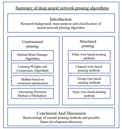
As early as 1990, Lecun et al. [4] proposed removing the small-contributing parameters from neural networks. This can not only decrease the network's computational complexity but also enhance its generalization ability and solve the problem of overfitting. Pruning is one of the standard methods for compressing neural networks, as it can remove many low-contributing parameters while maintaining the original accuracy of the network and reducing its computational complexity, thus achieving effective compression. Of course, besides pruning, there are many other methods for compressing networks, such as knowledge distillation [5] and quantization [6]. This article mainly .shortcomings of current pruning methods and possible future development directions in the end, as shown in figure1.

Methods for artificial pruning of neural networks can be broadly categorized into two types: unstructured pruning and structured pruning. Unstructured pruning can prune specific weights, thereby increasing the sparsity of the model. On the other hand, structured pruning has a larger granularity and prunes kernels or channels, but this changes the original structure of the network, hence the name "structured pruning."

2. Unstructured pruning

Non-structured pruning appeared early. As early as 1990, Lecun et al. [4] proposed the optimal brain damage (OBD) method, which is also an early pruning method based on connection importance. They established a local model of the error function and deleted parameters through Taylor expansion to reduce network size and improve generalization. However, although OBD hypothetically ignored the off-diagonal terms of the Hessian matrix, it still needs to calculate part of the Hessian matrix, which undoubtedly dramatically increases the computational cost of optimization.

Han et al. [7] proposed to prune the network by learning to find essential connections. Iteratively removing the connections with weights below a certain threshold from the network can significantly reduce the number of neurons in the final network. Han et al. additionally integrated quantization and Huffman coding to further compress the model, shrinking the parameter count of the ImageNet-trained VGG16 model from 138M to 11.3M. However, the above methods require much time and exceptional hardware support.

Generally, regularization-based pruning methods constrain the network parameter count during the training process with norms. Among norms, the \( {L_{0}} \) norm is one of the most basic norms, which denotes

\( {‖x‖_{0}}=cnt\lbrace i|x(i)≠0\rbrace \ \ \ LISTNUM NumberDefault \l 4 \)

In the formula, \( cnt \) represents the number of elements in the \( \lbrace i|x(i)≠0\rbrace \) , and \( x \) represents a vector, so \( {L_{0}} \) norm represents the quantity of non-zero elements in \( x \) . However, the \( {L_{0}} \) norm cannot be derived, making it unusable in normal circumstances. Typically, it is approximated by other norms, and the \( {L_{1}} \) and \( {L_{2}} \) norms are commonly used. The \( {L_{1}} \) norm is as follows

\( {‖x‖_{1}}=\sum _{i}|{x_{i}}|\ \ \ LISTNUM NumberDefault \l 4 \)

The \( {L_{1}} \) norm of a vector \( x \) is the total of the absolute values of all its elements. The \( {L_{1}} \) norm is defined as follows:

\( {‖x‖_{2}}=\sqrt[]{\sum _{i}{|{x_{i}}|^{2}}}\ \ \ LISTNUM NumberDefault \l 4 \)

Louizos et al. [8] proposed using variational optimization theory to make the introduction of \( {L_{0}} \) loss function differentiable, thereby solving the problem that the \( {L_{0}} \) norm cannot be derived.

In 2018, Zhang et al. [9] suggested a technique that transformed the weight pruning challenge of neural networks into a problem about constrained non-convex optimization and employed the Alternating Direction Method of Multipliers algorithm for network pruning.

Although unstructured pruning increases the sparsity of the network by directly removing parameters while maintaining the network's original accuracy, its effectiveness is often limited in practical scenarios. Firstly, storing sparse matrices in the network incurs additional memory costs. Secondly, there is currently a scarcity of software and hardware platforms that can efficiently perform sparse matrix operations, which makes it challenging to replicate the experimental findings reported in the literature. Finally, optimizing the network demands a considerable amount of time and resources.

3. Structured pruning

In recent years, convolutional neural networks (CNNs) have become ubiquitous in deep learning. While unstructured pruning can effectively reduce the size of neural networks to some extent, it faces particular challenges when applied to convolutional neural networks, including the following issues:

• Unstructured pruning usually needs to consider and prune each weight separately. This may lead to the irregular distribution of residual weights, thus destroying local connection characteristics and weight sharing in convolutional neural networks.

• Unstructured pruning may destroy the sparsity of convolution operations in convolutional neural networks, resulting in reduced efficiency of convolution operations.

• Convolutional neural networks typically contain a high concentration of parameters within the fully connected layer. These parameters are usually unsuitable for unstructured pruning because there is a dense connection between these parameters. However, unstructured pruning cannot handle this dense connection.

Therefore, structured pruning is usually used for the pruning of convolutional neural networks. This method can maintain the sparsity and local connection characteristics of convolutional neural networks and can competently deal with the problem of parameter-dense connection in the fully connected layer.

This paper divides structured pruning into Filter-wise, Channel-wise, Group-wise, and Stripe-wise. Next, these four pruning methods will be introduced and compared.

3.1. Filter-wise pruning

Convolution kernel pruning is an essential structured pruning method that reduces the computational complexity and the number of network parameters by deleting some convolution kernels with small contributions in the network and maintaining the network performance as much as possible. The following will introduce four typical convolution kernel pruning algorithms.

In a matrix, the rank of the matrix often represents the amount of information carried by the matrix. Lin et al. [10] found that it is the same that a specific convolution kernel generates multiple feature maps’ average ranks. After experimental verification, the larger the rank of the feature map, the more information it contains. So, they proposed the HRank method. The importance of different convolution kernels in the model is obtained by analyzing the rank of the feature map. Finally, the convolution kernels that generate low-rank feature maps are cut off to achieve the compression model effect.

ThiNet [11] is a pruning method based on accelerated sparse convolutional neural networks proposed by Luo et al.. The central concept is to prune the convolutional neural network by examining the redundancy among feature maps to decrease the computational and storage requirements of the network. In contrast to conventional pruning methods, ThiNet utilizes a novel index termed "feature reuse rate" to gauge the extent of reuse of each filter in the convolution layer across distinct feature maps. Specifically, ThiNet first clusters the input data to gather similar data together and then obtains a sub-sampled data set by sub-sampling the data of each cluster. Then, for each filter in the convolution layer, the correlation and feature reuse rate between it and other convolution kernels are calculated, and the convolution kernels are sorted according to these indicators. Then, by pruning the filter with a low reuse rate, the computation and storage of the network can be reduced.

In 2018, He et al. [12] considered that much previous work was Hard Filter Pruning, that is, deleting convolution kernels directly and unrecoverable, which may reduce the network's learning ability. Therefore, they proposed Soft Filter Pruning ( SFP ). Precisely, the \( {L_{p}} \) norm is calculated during the \( k \) round of training, and then the filter with a smaller \( {L_{p}} \) norm is set to zero, and then the \( k+1 \) round of training is performed. After updating the weights in the filter by error backpropagation, the \( {L_{p}} \) norm and zeroing operations are repeated until the end of training. Finally, the filter with a smaller \( {L_{p}} \) norm is pruned. This method dynamically adjusts the pruning of the filter during the training process so that the network accuracy after pruning is even higher than the original network.

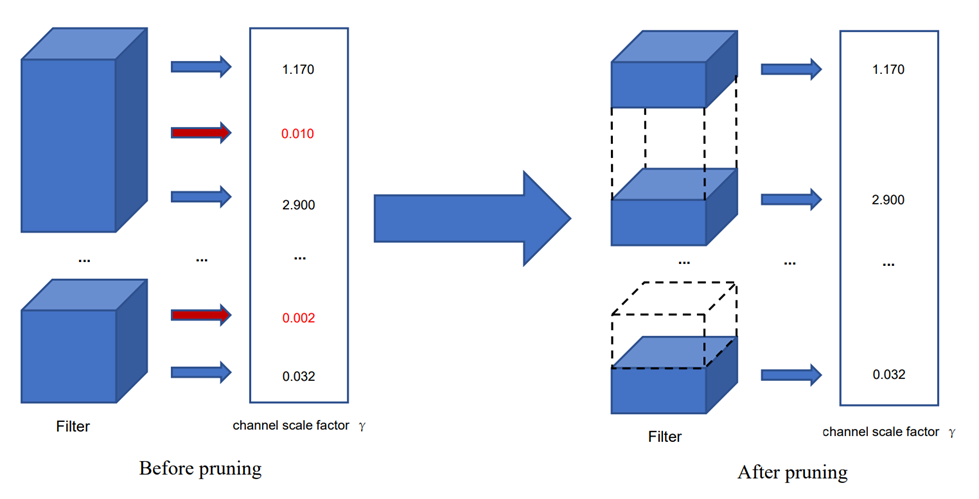
He et al. proposed the FPGM [13] algorithm in 2019, which compresses the model by pruning redundant filters instead of convolution kernels with relatively minor importance. The primary concept of the FPGM algorithm is to determine the significance of the filter by calculating the geometric median of each filter. In the training process, the FPGM algorithm sorts the convolution kernels according to the geometric median of the filters and deletes a certain proportion of the less critical filters. The FPGM algorithm does not entirely use norm-based pruning criteria for pruning, which can more accurately evaluate the importance of each filter and has a good pruning effect (Figure 2).

3.2. Channel-wise pruning

Channel pruning compresses the network by removing channels with little contribution and unimportant information in the neural network. The following will introduce several typical channel pruning methods (Table 1).

Table 1. shows the comparison of pruning algorithms. All these tests' dataset is CIFAR-10. Top-1 refers to the accuracy of the category with the highest prediction probability in line with the actual results.

Liu et al. [14] proposed that each channel in the network can be optimized by introducing a scaling factor. Specifically, each channel is multiplied by a scaling factor. Then these factors are added to the network training, which is regularized to achieve the purpose of sparse factors. According to this idea, the loss function of network training is defined as

\( L=\sum _{(x,y)}loss(f(x,w),y)+λ\sum _{γ∈Γ}g(γ)\ \ \ LISTNUM NumberDefault \l 4 \)

The first half of the loss function is the loss of network output and label, where \( x \) is the network input and \( y \) is the training label. The latter part is the loss caused by the regularization of the channel factor, where \( γ \) is the channel scaling factor, and \( g \) represents a regularization norm. In the author's paper, the \( {L_{1}} \) norm is used, and \( λ \) is a hyperparameter.

After training, the channel scaling factor \( γ \) in the network will change with the iteration of the network. When \( γ \) is small, it indicates that the importance of the current channel is low. Therefore, the channel with a small channel factor can be selected to delete to achieve the effect of reducing network size and position accuracy.

The original essay's channel scale factor comes from the BN layer's scale factor [15]. The BN layer is as follows:

\( \hat{z}=\frac{{z_{in}}-{μ_{B}}}{\sqrt[]{σ_{B}^{2}+ϵ}}; {z_{out}}= γ\hat{z}+β\ \ \ LISTNUM NumberDefault \l 4 \)

Where \( {z_{in}} \) is the BN layer input, \( {μ_{B}} \) is the input mean, \( σ_{B}^{2} \) is the input variance, \( {z_{out}} \) is the BN layer output, \( γ \) and \( β \) are trainable parameters, where \( γ \) is the scale factor, which is directly used as the channel scale factor and used to judge the importance of the channel. However, Huang and Wang [16] improved the method since some networks may not have a BN layer. They proposed introducing additional scale factors to make the method more general.

Although the above-proposed method is effective, it needs to train the entire network from scratch when pruning the network, which may generate much extra time overhead. Therefore, there is also a pruning algorithm for the trained model, which only needs to fine-tune the network after pruning.

Polyak and Wolf [17] argued that an input channel has different contributions to the output of different convolution kernels, so they proposed a method based on eliminating low-activity channels, calculating the variance of the output value of each channel, and using the variance as the channel activity index. Specifically, for a convolutional layer \( t \) with input \( X \) , output \( Y \) , weight \( W \) , and depth \( m \) , there are

\( {Y_{t}}=\sum _{s=1}^{m}{W_{ts}}*{X_{s}}\ \ \ LISTNUM NumberDefault \l 4 \)

Therefore, the channel activity from the convolution kernel \( t \) comes from \( {W_{ts}}*{X_{s}} \) , so its variance can be calculated as

\( {σ_{ts}}=var(‖{W_{ts}}*{X_{s}}‖F)\ \ \ LISTNUM NumberDefault \l 4 \)

The larger the variance, the richer the features learned by the channel and the more significant the contribution to the results. By setting a threshold, the less active channels are deleted, which can effectively reduce the network's computation and storage.

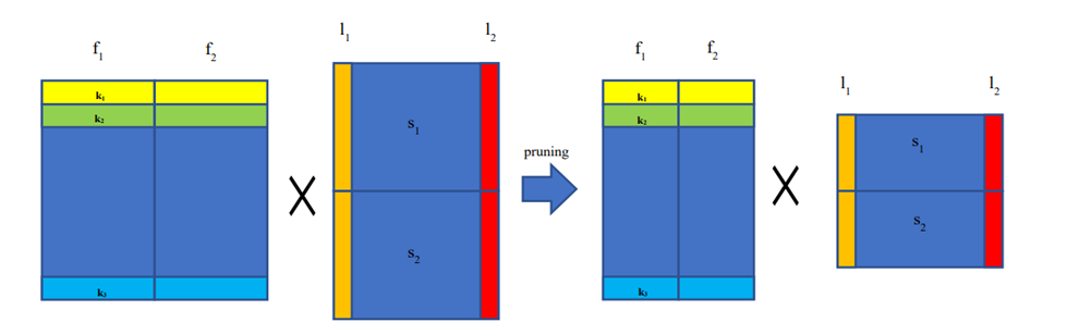
There is also a class of channel pruning algorithms based on machine learning methods and search algorithms to find excellent network compression structures. Hu et al. [18] proposed that the channel pruning algorithm can be regarded as a combinatorial optimization problem with exponential solution space, which a genetic algorithm can solve. In order to improve the search efficiency of the genetic algorithm, a two-step approximate fitness function is designed. Chang et al. [19] divided the optimization process into four parts. Firstly, clustering was performed by the resemblance of feature maps for initial pruning. Secondly, by employing the population initialization technique to convert the network structure into a set of candidate populations. These populations are then subject to a search process based on particle swarm optimization to identify the optimal compression structure. Finally, the pruned network undergoes a fine-tuning phase (Figure 3).

3.3. Group-wise pruning

Implementing most convolution operations is not as direct as it seems to slide the convolution kernel on the input channel because such a calculation method is challenging to optimize the acceleration, and it is easier to optimize the acceleration by converting it into matrix multiplication. On the one hand, the operation data is stored in persistent memory after transforming into a matrix, which is convenient for hardware optimization acceleration, such as cache. On the other hand, many libraries implement efficient matrix multiplication, such as BLAS [20], which can significantly accelerate the operation speed.

The group-wise pruning prunes the exact position of a set of convolution kernels. This pruning method can fully use the operation mentioned above through the structured sparse convolution kernel to compress the matrix and achieve the acceleration effect. Because of its small pruning granularity, it can achieve a good compression effect.

In 2016, Lebedev and Lempitsky [21] proposed a pruning method based on Group-wise. They believed that the matrix multiplication method of convolution calculation mentioned above could be used to achieve accelerated calculation. They considered two optimization processes at the same time. The first one is to sparse the model during training, and the second is to sparse the trained model. For the first optimization process, they add a group-sparse regularizer based on the \( {L_{2,1}} \) norm to the gradient loss of the network so that the network can generate a specific group sparse structure. For the second optimization process, they adopted the Gradual Group-wise Sparsification method. Specifically, they selected groups with small regularization terms by setting a specific threshold for sparseness, reducing damage to the critical part of the network after the neural network is structured sparsely in the form shape-wise, and the matrix operation of the convolution changes.

After deleting a set of convolution kernels with parameters at the same position, the convolution kernel participating in matrix operation becomes smaller, thus realizing network acceleration. It is affected, thereby reducing the damage of sparseness to essential parts of the network by setting the hold-out set to maintain.

In ' Learning Structured Sparsity in Deep Neural Networks ' [22], Wen et al. summarized the optimization goal of Group-wise pruning as follows :

\( E(W)={E_{D}}(W)+{λ_{s}}∙\sum _{l=1}^{L}(\sum _{{c_{l}}=1}^{{C_{l}}}\sum _{{m_{l}}=1}^{{M_{l}}}\sum _{{k_{l}}=1}^{{K_{l}}}{‖W_{:,{c_{l}},{m_{l}},{k_{l}}}^{(l)}‖_{g}})\ \ \ LISTNUM NumberDefault \l 4 \)

Where \( {E_{D}}(W) \) denotes the prediction loss, \( \sum _{l=1}^{L}(\sum _{{c_{l}}=1}^{{C_{l}}}\sum _{{m_{l}}=1}^{{M_{l}}}\sum _{{k_{l}}=1}^{{K_{l}}}{‖W_{:,{c_{l}},{m_{l}},{k_{l}}}^{(l)}‖_{g}}) \) is the regularization of the weight of the group lasso paradigm, \( {λ_{s}} \) is the regularization factor, the purpose is to balance the two items.

Later, in 2019, Wang et al. [23] believed that the fixed-size regularization factor usually used in the previous method ignores the sensitivity of the CNN network and may cause damage to the CNN network. Therefore, they improved the optimization goal and proposed a dynamic regularization method. Specifically, they introduced unstructured regularization terms and group lasso regularization terms into the optimization goal and weighted them with dynamic regularization factors. This method has a very high acceleration rate and a minimal accuracy decline among many methods at that time.

3.4. Stripe-wise pruning

The pruning methods mentioned above almost consider the importance of different parameters in the neural network, while Stripe-wise pruning is based on the consideration of filter shape.

Meng et al. [24] proposed this method in their paper 'PRUNING FILTER IN FILTER' published in 2020. They implicitly learned the better shape of the filter by introducing Filter Skeleton into the convolution layer during training. Specifically, they describe the loss function as

\( L=\sum _{(x,y)}loss(f(x,W⊙I),y)\ \ \ LISTNUM NumberDefault \l 4 \)

Among them, \( ⊙ \) represents the point multiplication operation, \( W \) represents the weight in the convolution layer, and \( I \) represent Filter Skeleton. I hope to learn the different Stripes' importance by adding Filter Skeleton to gradient descent. However, this alone does not filter out some Stripes with less contribution well, so the author adds a regularization term to the loss function to sparse the filter Skeleton and achieves a better filtering result.

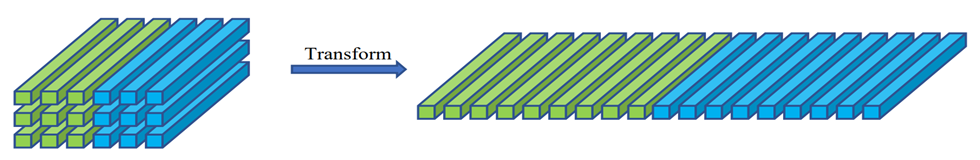
After learning the better shape of the filter through Filter Skeleton, some Stripes are deleted, but this will destroy the structure of the convolution. The author uses the method of reorganizing the filter. They transform the original N filters with a size of \( K*K \) into \( N*K*K \) filters with a size of \( 1*1 \) , as shown in Figure 4.

After this operation, the shape learned by the previous Filter Skeleton can be used to delete some filters to achieve the effect of compressing the model. Since this method solely prunes at the Stripe level, it can preserve high performance without requiring fine-tuning. Additionally, it can achieve a high pruning rate due to its small pruning granularity.

4. Conclusion and discussion

The primary purpose of pruning is to decrease the parameters of a network and expedite network computations. In this paper, the pruning algorithms of neural networks in recent years are classified and summarized. The unstructured pruning algorithm and the structured pruning algorithm are introduced. According to the pruning granularity and starting point, the structured pruning algorithms are divided into four categories: Filter-wise pruning、Group-wise pruning、Stripe-wise pruning, and Channel-wise pruning.

Unstructured pruning can delete the parameters with negligible contribution from the neural network to the greatest extent. However, it needs the support and optimization of hardware and library to exert its advantages.

Compared with unstructured pruning, structured pruning has a larger granularity, which can optimize the network's structure and does not need additional hardware and library support because it directly reduces parameters. The main disadvantage is that the change of input and output dimensions in the middle layer of the network may cause profound accuracy loss or some deviation to the network, and even the disappearance of the middle layer of the network may occur.

The practical and easy-to-implement structured pruning algorithms are mainly about convolutional neural networks. However, with the popularity of language processing models such as ChatGPT in recent years, it can be predicted that natural language processing tasks will receive more attention. As the backbone network of most language processing models, Transformer [25] has excellent context processing capabilities and heavy parameters and calculations to neural networks. Therefore, implementing an algorithm that can effectively compress the Transformer skeleton network will be a promising direction.

In addition, graph neural networks are more in line with the human brain structure in theory and may have significant development in the future. However, there are few pruning algorithms for neural graph networks, so that pruning algorithms can be developed for such networks in the future.

Several automated network structure search algorithms have emerged, such as the SPOS [26] and the ENAS algorithm [27]. They are committed to finding the optimal network sub-model through search algorithms, simplifying the network structure.

References

[1]. K. Simonyan and A. Zisserman, “Very Deep Convolutional Networks for Large-Scale Image Recognition.” arXiv, Apr. 10, 2015. doi: 10.48550/arXiv.1409.1556.
[2]. K. He, X. Zhang, S. Ren, and J. Sun, “Deep Residual Learning for Image Recognition,” in 2016 IEEE Conference on Computer Vision and Pattern Recognition (CVPR), Las Vegas, NV, USA, Jun. 2016, pp. 770–778. doi: 10.1109/CVPR.2016.90.
[3]. G. Huang, Z. Liu, L. van der Maaten, and K. Q. Weinberger, “Densely Connected Convolutional Networks.” arXiv, Jan. 28, 2018. Accessed: Feb. 19, 2023. [Online]. Available: http://arxiv.org/abs/1608.06993
[4]. Y. Lecun, “Optimal Brain Damage,” Neural Information Proceeding Systems, vol. 2, no. 279, pp. 598–605, 1990, doi: http://dx.doi.org/.
[5]. J. Gou, B. Yu, S. J. Maybank, and D. Tao, “Knowledge Distillation: A Survey,” Int J Comput Vis, vol. 129, no. 6, pp. 1789–1819, Jun. 2021, doi: 10.1007/s11263-021-01453-z.
[6]. A. Gholami, S. Kim, Z. Dong, Z. Yao, M. W. Mahoney, and K. Keutzer, “A Survey of Quantization Methods for Efficient Neural Network Inference.” arXiv, Jun. 21, 2021. Accessed: Mar. 06, 2023. [Online]. Available: http://arxiv.org/abs/2103.13630
[7]. S. Han, J. Pool, J. Tran, and W. Dally, “Learning both Weights and Connections for Efficient Neural Network”.
[8]. C. Louizos, M. Welling, and D. P. Kingma, “Learning Sparse Neural Networks through $L_0$ Regularization.” arXiv, Jun. 22, 2018. doi: 10.48550/arXiv.1712.01312.
[9]. X. Zhang, X. Zhou, M. Lin, and J. Sun, “ShuffleNet: An Extremely Efficient Convolutional Neural Network for Mobile Devices,” in 2018 IEEE/CVF Conference on Computer Vision and Pattern Recognition, Salt Lake City, UT, Jun. 2018, pp. 6848–6856. doi: 10.1109/CVPR.2018.00716.
[10]. M. Lin et al., “HRank: Filter Pruning Using High-Rank Feature Map,” in 2020 IEEE/CVF Conference on Computer Vision and Pattern Recognition (CVPR), Seattle, WA, USA, Jun. 2020, pp. 1526–1535. doi: 10.1109/CVPR42600.2020.00160.
[11]. J.-H. Luo, J. Wu, and W. Lin, “ThiNet: A Filter Level Pruning Method for Deep Neural Network Compression,” in 2017 IEEE International Conference on Computer Vision (ICCV), Venice, Oct. 2017, pp. 5068–5076. doi: 10.1109/ICCV.2017.541.
[12]. Y. He, G. Kang, X. Dong, Y. Fu, and Y. Yang, “Soft Filter Pruning for Accelerating Deep Convolutional Neural Networks,” in Proceedings of the Twenty-Seventh International Joint Conference on Artificial Intelligence, Stockholm, Sweden, Jul. 2018, pp. 2234–2240. doi: 10.24963/ijcai.2018/309.
[13]. Y. He, P. Liu, Z. Wang, Z. Hu, and Y. Yang, “Filter Pruning via Geometric Median for Deep Convolutional Neural Networks Acceleration,” in 2019 IEEE/CVF Conference on Computer Vision and Pattern Recognition (CVPR), Long Beach, CA, USA, Jun. 2019, pp. 4335–4344. doi: 10.1109/CVPR.2019.00447.
[14]. Z. Liu, J. Li, Z. Shen, G. Huang, S. Yan, and C. Zhang, “Learning Efficient Convolutional Networks through Network Slimming,” in 2017 IEEE International Conference on Computer Vision (ICCV), Venice, Oct. 2017, pp. 2755–2763. doi: 10.1109/ICCV.2017.298.
[15]. S. Ioffe and C. Szegedy, “Batch Normalization: Accelerating Deep Network Training by Reducing Internal Covariate Shift”.
[16]. Z. Huang and N. Wang, “Data-Driven Sparse Structure Selection for Deep Neural Networks,” in Computer Vision – ECCV 2018, vol. 11220, V. Ferrari, M. Hebert, C. Sminchisescu, and Y. Weiss, Eds. Cham: Springer International Publishing, 2018, pp. 317–334. doi: 10.1007/978- 3-030-01270-0_19.
[17]. A. Polyak and L. Wolf, “Channel-level acceleration of deep face representations,” IEEE Access, vol. 3, pp. 2163–2175, 2015, doi: 10.1109/ACCESS.2015.2494536.
[18]. Y. Hu, S. Sun, J. Li, X. Wang, and Q. Gu, “A novel channel pruning method for deep neural network compression.” arXiv, May 29, 2018. doi: 10.48550/arXiv.1805.11394.
[19]. J. Chang, Y. Lu, P. Xue, Y. Xu, and Z. Wei, “ACP: Automatic Channel Pruning via Clustering and Swarm Intelligence Optimization for CNN.” arXiv, Jan. 16, 2021. Accessed: Feb. 21, 2023. [Online]. Available: http://arxiv.org/abs/2101.06407
[20]. “An updated set of basic linear algebra subprograms (BLAS),” ACM Trans. Math. Softw., vol. 28, no. 2, pp. 135–151, Jun. 2002, doi: 10.1145/567806.567807.
[21]. V. Lebedev and V. Lempitsky, “Fast ConvNets Using Group-Wise Brain Damage,” in 2016 IEEE Conference on Computer Vision and Pattern Recognition (CVPR), Las Vegas, NV, USA, Jun. 2016, pp. 2554–2564. doi: 10.1109/CVPR.2016.280.
[22]. W. Wen, C. Wu, Y. Wang, Y. Chen, and H. Li, “Learning Structured Sparsity in Deep Neural Networks.” arXiv, Oct. 18, 2016. Accessed: Feb. 21, 2023. [Online]. Available: http://arxiv.org/abs/1608.03665
[23]. H. Wang, Q. Zhang, Y. Wang, Y. Lu, and H. Hu, “Structured Pruning for Efficient ConvNets via Incremental Regularization.” arXiv, Apr. 15, 2019. Accessed: Feb. 21, 2023. [Online]. Available: http://arxiv.org/abs/1804.09461
[24]. F. Meng et al., “Pruning Filter in Filter.” arXiv, Dec. 09, 2020. doi: 10.48550/arXiv.2009.14410.
[25]. A. Vaswani et al., “Attention Is All You Need.” arXiv, Dec. 05, 2017. Accessed: Mar. 05, 2023. [Online]. Available: http://arxiv.org/abs/1706.03762
[26]. Z. Guo et al., “Single Path One-Shot Neural Architecture Search with Uniform Sampling.” arXiv, Jul. 08, 2020. doi: 10.48550/arXiv.1904.00420.
[27]. H. Pham, M. Y. Guan, B. Zoph, Q. V. Le, and J. Dean, “Efficient Neural Architecture Search via Parameter Sharing.” arXiv, Feb. 11, 2018. doi: 10.48550/arXiv.1802.03268.
Cite this article
Ling,X. (2023). Summary of Deep Neural Network Pruning Algorithms. Applied and Computational Engineering,8,334-343.
Data availability
The datasets used and/or analyzed during the current study will be available from the authors upon reasonable request.
Disclaimer/Publisher's Note
The statements, opinions and data contained in all publications are solely those of the individual author(s) and contributor(s) and not of EWA Publishing and/or the editor(s). EWA Publishing and/or the editor(s) disclaim responsibility for any injury to people or property resulting from any ideas, methods, instructions or products referred to in the content.
About volume
Volume title: Proceedings of the 2023 International Conference on Software Engineering and Machine Learning
© 2024 by the author(s). Licensee EWA Publishing, Oxford, UK. This article is an open access article distributed under the terms and
conditions of the Creative Commons Attribution (CC BY) license. Authors who
publish this series agree to the following terms:
1. Authors retain copyright and grant the series right of first publication with the work simultaneously licensed under a Creative Commons
Attribution License that allows others to share the work with an acknowledgment of the work's authorship and initial publication in this
series.
2. Authors are able to enter into separate, additional contractual arrangements for the non-exclusive distribution of the series's published
version of the work (e.g., post it to an institutional repository or publish it in a book), with an acknowledgment of its initial
publication in this series.
3. Authors are permitted and encouraged to post their work online (e.g., in institutional repositories or on their website) prior to and
during the submission process, as it can lead to productive exchanges, as well as earlier and greater citation of published work (See
Open access policy for details).