1. Introduction

Stock is a share of the assets of an organization which have some value or price associated with it. The place where stocks are made available to the public is known as stock market. Investors usually trade on the market by buying and selling stocks with the aim of making profit when the price goes higher than it was purchased [1].

Predicting the direction of price movement with some accuracy is necessary to determine buying and selling stock. Investors focus on stock price prediction in order to yield significant profits. Traditional stock price prediction methods include technical analysis, fundamental analysis and time series. The technical analysis use historical price movement to predict price pattern while the fundamental analysis use the financial information about the company such as inventory or revenue growth relates [2]. Time series method involves using historical performance for prediction with current observations dependent on past observation in time [3]. However, it sometimes fails to accurately forecast the financial market because of national and global economic trends [4].

Deep learning (DL) models are recent methods that have also successfully analyzed time series data more accurately when compared to the other traditional methods [5], [6]. The DL models is able to learn complex mappings of multiple inputs and outputs. The work aims to develop a model based on LSTM and multivariate time series to predict stock price. The work is introduced in Section 1. Section 2 presents some related works. The methodology for the proposed model is discussed in section 3. The experiments and analysis of the model is discussed in section 4. Finally, the work is concluded in in Section 5.

2. Literature review

A review of existing research work on stock prediction using machine learning techniques is discussed. Gozalpour and Teshnehlab [7] proposed the closing price prediction model using Jordan Recursive Neural Network (JRNN) model. Data used on the model include Microsoft Corporation, NAS-DAQ symbols, Intel Corporation and National Bank shares Inc. between 2007 and 2017. The model was evaluated with the results shows a MAPE for all symbols with less than 3%. A stock prediction method is proposed in in [8] to predict stock price using Elman neural network (ENN). The study optimized the parameter of the model using Grey Wolf optimization (GWO) algorithm.

Model evaluation is testing out on NYSE and NASDAQ data. The results show the proposed model provides high accurate predictions. Ingle and Deshmukh [9] propose a framework for stock market data prediction. The framework use GLM, GBM, Deep learning with PCA, PCR, k- Means models. The model use data of Bombay Stock Exchange to achieve an accuracy of approximately 85%.

Huynh et al. [10] introduce a model that applies LSTM and GRU models to predict and classify stock price movements. The experiment use Reuters and Bloomberg financial news combined with Yahoo Finance price data to forecasting (S&P500) index. Wu et al. [11] propose an integrated prediction method using bi-directional LSTM. The work considers the financial news corpus and the stock technical factors. The work used the dataset from Chinese market and news data for approximately four years. The proposed method achieves superior performance with low overfitting when compared with other baselines methods. Nikou et al. [12] used ANN, SVR, RF, and LSTM data mining techniques to predict close price. The dataset used in the work include the close price of iShares MSCI United Kingdom exchange‐traded fund. The results indicates that that the LSTM method functions better in predicting the close price better than the other methods. Pang et al. [13] use LSTM-based prediction method with embedded layer (ELSTM) and based on automatic encoder (AELSTM). Stock historical data used in the implementation includes stock data of the Shanghai A-share market and Shenzhen stock market. Nabipour et al. [14] employed LSTM to predict stock market of Iran. The work use dataset of Petroleum, Non-metallic minerals, Diversified Financials and Basic metals stock market groups. The result shows more accuracy when compared with other learning methods. In [15], Long Short-term memory methods is used with Auto Regressive Integrated Moving Average (ARIMA). Daily EUR/USD exchange rates is used for implementation. The LSTM method produced a better prediction result compared to the ARIMA.

Vargas et al. [16] presented a hybrid Recurrent Neural Networks (RNN) and Convolutional Neural Networks (CNN) technique for stock price movement prediction. Financial news title with technical indicators are used to predicts intraday directional movements using the Standard & Poor’s 500 (S&P500) dataset. The implementation result shows some improvement compared with other works. In [17], Long Short-term Memory (LSTM) and Convolutional Neural Network (CNN) is used to predict stock price. The datasets used in the work include S&P500 and Dow Jones (DJIA). The proposed model achieves more accurate predictions than other traditional models. Chavan et al. [1] propose a CNN for predicting the stock price. The data consists of one year stock price of Apple company. Yang et al. [18] present a prediction technique by combining a CNN and LSTM network. The models are applied on S&P 500, DJIA, NASDAQ, NYSE, and RUSSELL stock indices.

3. Methodology

The methodology of the proposed technique makes use of the multivariate time series and LSTM model designs as described in the subsequent subsections.

3.1. Multivariate time series

This study obtains a multivariate time series from the stock historical dataset with a combination of more than one time-dependent variable. Let \( {x_{1}}(t),{x_{2}}(t),…,{x_{K}}(t) \) represent a set \( K \) independent variables with of the variable vector padded to a uniform length of \( N \) as shown in Equation 1.

\( x(t)=[{x_{1}},{x_{2}},…,{x_{N}}] \) (1)

where \( {x_{i}}(t) ∈{R^{N}} \) represent data point with n-dimensions at time \( t \) . The independent variable set is drawn from the same underline distribution over \( M \) datapoints to form a stack of \( K×M \) multivariate time series \( X \) as given in Equation 2.

\( X=[\begin{matrix}{x_{11}} & {x_{12}} & ⋯ & {x_{1K}} \\ {x_{21}} & {x_{22}} & ⋯ & {x_{2K}} \\ ⋯ & ⋯ & ⋯ & ⋯ \\ {x_{M1}} & {x_{M1}} & ⋯ & {x_{MK}} \\ \end{matrix}] \) (2)

Let vector \( y∈{R^{M}} \) representing \( M \) dependent variable vectors drawn from the same distribution as \( {x_{i}}(t) \) . The sequence of the label is also defined in Equation 3.

\( Y=[\begin{matrix}{y_{1}} \\ {y_{2}} \\ ⋯ \\ {y_{M}} \\ \end{matrix}] \) (3)

3.2. The LSTM neural network

The proposed LSTM model takes the time sequences xi as input and yield a predicted values y as output as shown in the structure shown in Fig. 1.

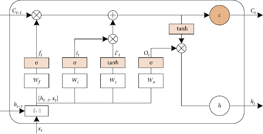
Figure 1. LSTM architecture.

The LSTM model calculates the predicted values using the input, forget, output and with cell candidate gates defined in Equation 4, Equation 5, Equation 6 and Equation 7 respectively:

\( {i_{t}}={σ_{g}}({W_{i}}{x_{t}}+{Q_{i}}{h_{t-1}}+ {b_{i}}) \) (4)

\( {f_{t}}={σ_{g}}({W_{f}}{x_{t}}+{Q_{f}}{h_{t-1}}+ {b_{f}}) \) (5)

\( {C_{t}}= {σ_{c}}({W_{c}}{x_{t}}+{Q_{c}}{h_{t-1}}+ {b_{c}}) \) (6)

\( {o_{t}}={σ_{t}}({W_{o}}{x_{t}}+{Q_{o}}{h_{t-1}}+ {b_{o}}) \) (7)

where \( {i_{t}} \) represent input gates, \( {o_{t}} \) represent the output gate, \( {f_{t}} \) is the forget gate, \( {C_{t}} \) is the cell candidate, \( {σ_{g}} \) is the gate activation function, \( W \) represent the input weight. \( R \) represent the recurrent weight matrices. \( {x_{t}} \) represent the input vector, and \( {h_{t-1}} \) is the input at the previous time ( \( t-1) \) . \( b \) represent the bias vector. The forget gate chooses the prior information to be remembered or forgotten. The cell learns new information, at the input gate, from the input while the output gate passes the updated information from one timestamp to the next. The cell state \( {C_{t}} \) and the output \( {h_{t}} \) at time \( t \) are determined as shown in Equation 8 and Equation 9 respectively:

\( {c_{t}}={f_{t}}*{c_{t-1}}+{i_{t}}*{g_{t}} \) (8)

\( {h_{t}}={o_{t}}*{σ_{c}}({c_{t}}) \) (9)

where * denotes the Hadamard product (element-wise multiplication of vectors).

3.3. Data description and preprocessing

The study employed historical dataset of First Bank of Nigeria Holdings (FBNH) stock in Nigerian Stock market Index from January, 2014 to March 2022. The dataset is obtained online from Capital Asset Ltd, a stockbroking firm with the Nigerian Stock Exchange (NSE), with the URL: www.capitalassetsng.com. The dataset is made up of 1,977 rows and 9 columns. The rows are daily stock transactions listed under the columns: prev close, open, high, low, close, trades, volume, value and date. Features defined from the fields are used to predict the closing price of the next trading day as output. The closing price of the stock between 2014 and 2022 is shown in Fig. 2.

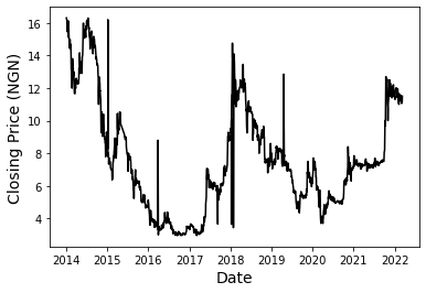
Figure 2. Closing price of the FBNH stock.

The features is defined using previous close, open, high, low, trades, volume and value. The target is defined as the closing price. During the preprocessing the data is normalized and rescaled within a fixed range [0,1] to avoid features with larger value from unjustly interfering and biasing the model and to achieve rapid convergence. The data is also resized to 2D matrix to make it better suited for the deep network training.

3.4. Train, test and validation sets

The dataset is split into train, test and validation sets. The ratio of the train to test split is 90:10 while the train to validation ratio is 80:20. The training set is used to train and make the model learn the hidden patterns in the data. Both the input and output of the training set is used to fit the model. The validation set is used to evaluate the model by fine-tuning the model hyperparameters such as the number of hidden units. Exactly 20 percent of the train data is the validation. The evaluation of the proposed model is carried out using test data after fitting the model using the train and validation sets. In the testing stage, the input element of the testing dataset is provided to the model and predictions are make and compared to the expected values.

4. Results and discussion

4.1. Performance measures

The accuracy of the prediction is measured using metric that includes the mean absolute percentage error (MAPE), mean absolute error (MAE) and root mean square error (RMSE). The execution time for the implementation is also obtained. Mean absolute percentage error is calculated by taking the difference between the actual value and the predicted value and dividing it by the actual value. An absolute percentage is applied to this value and it is averaged across the dataset. The smaller the MAPE, the better the model performance as shown in Equation 10.

\( MAPE=\frac{1}{n}\sum _{i=1}^{n}|\frac{{y_{i}}-y_{i}^{ \prime }}{{y_{i}}}|×100 \) (10)

Where n is the sample size, \( {y_{i}} \) is the actual data value and \( y_{i}^{ \prime } \) is the predicted data value.

The average magnitude of errors of the prediction is gives the mean absolute error measures. The lower the MAE, the higher the accuracy of a model. Mathematically, MAE can be expressed as shown in Equation 11.

\( MAE=\frac{1}{n}\sum _{i=1}^{n}|{y_{i}}-y_{i}^{ \prime }| \) (11)

Where \( {y_{i}} \) is the observed value for the \( {i^{th}} \) observation, \( y_{i}^{ \prime } \) is the predicted value for the \( {i^{th}} \)  observation and n is the total number of observations. Mean Squared Error (MSE) measures the the average squared difference between the target variable and the predicted value (see Equation 12):

\( MSE=\frac{1}{n}\sum _{i=1}^{n}{({y_{i}}-y_{i}^{ \prime })^{2}} \) (12)

Where n is the sample size, \( {y_{i}} \) is the actual data value and \( y_{i}^{ \prime } \) is the predicted data value. Relative Root Mean Square Error (RRMSE) is the root mean squared error normalized by the root mean square value where each residual is scaled against the actual value as defined in Equation 13:

\( RMSE=\sqrt[]{\frac{\frac{1}{n}\sum _{i=1}^{n}{({y_{i}}-y_{i}^{ \prime })^{2}}}{\sum _{i=1}^{n}{(y_{i}^{ \prime })^{2}}}} \) (13)

4.2. Hyperparameter optimization

The proposed model requires certain model parameters to train optimally. These parameters include number of layers, dimension of the input variable and activation function. The initial values of these parameter are as shown in Table 1. Extensive experiments are carried out to find the optimal parameter values for the model.

Table 1. Initial parameters.

The number of the LSTM unit specifies the capability of the network to memorize the information and correlate it with the past information. The result of the variations of the LSTM unit shows an optimum value of 200 units as shown in Table 2.

Table 2. Effect of LSTM units.

The batch size refers to the number of samples used to train a model before updating the weights and biases. The model was, thus, tested with different batch sizes as shown in Table 3. The optimal value for batch size was obtained with the batch size 10.

Table 3. Effect of batch size.

The epoch is used to determine the number of times the training process is repeated using the same training data. Choosing the right value will assist the model to converged and avoid the problem of overfitting. The optimum result is reached at epoch 150 as shown in Table 4.

Table 4. Effect of epochs.

The activation function ensures the model learns the training dataset well. The results from applying the common activation functions shows that Rectified linear activation function (ReLU) gives the best result as shown in Table 5.

Table 5. Effect of activation function.

The optimization algorithms is used to reduce the losses and providing the most accurate results possible. The optimization parameters considered include adagrad, adadelta, SGD, RMSprop and Adam. The results for various optimization techniques are shown in Table 6. From the result is seen that the Adam optimization parameter gives the best performance.

Table 6. Effect of optimization.

The implementation of proposed model is carried out using the optimized hyperparameter settings in Table 7. The predicted stock price is obtained for 179 test input data points over a period of 8 months. The predicated values are plotted against the actual outputs as shown in in Fig. 3.

Table 7. Optimized hyperparameter settings.

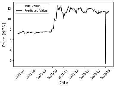
Figure 3. Actual vs predicted stock price.

It is observed that the prediction has lower error and higher accuracies in the first 3 months within the smoother trend in the trading price change. The performance evaluation is also carried out with other machine learning algorithms applied on same dataset. The comparison is as shown in Table 8. The proposed model outperforms the other models on mape, rmse and rrmse performance metric values.

Table 8. Comparison between traditional and proposed techniques.

5. Conclusion

In this study, a LSTM-based deep learning model is used to predict stock price using multivariate time series. The dataset is obtained from the historical data of First Bank of Nigeria Holdings. The technique creates a multivariate time series from the dataset using previous close, open, high, low, trades, volume and value. The dataset is split into train and test sets for model fitting and evaluation respectively. During the implementation the closing stock price is predicted and the accuracy is measured based on MAPE, MAE, RMSE, rRMSE metrics. The result is compared with other traditional machine learning methods and shows the proposed model performs best on mape, rmse, rrmse.

References

[1]. Chavan, S., Doshi, H., Godbole, D., Parge, P. & Gore, D.: 1D Convolutional Neural Network for Stock Market Prediction using Tensorflow. International Journal of Innovative Science and Research Technology, 4, 272–275 (2019).
[2]. Huang, C. J., Chen, P. W. & Pan, W. T.: Using multi-stage data mining technique to build forecast model for Taiwan stocks. Neural Computing and Applications, 21, 2057–2063 (2012).
[3]. Neto, M. C. A., Calvalcanti, G. D. C. & Ren, T. I. Financial time series prediction using exogenous series and combined neural networks. International Joint Conference on Neural Networks, 149–156 (2009).
[4]. Hsu, M. W., Lessmann, S., Sung, M. C., Ma, T. & Johnson, J. E. V.: Bridging the divide in financial market forecasting: machine learners vs. financial economists. Expert Systems with Application, 61, 215–234 (2016).
[5]. Sezer, O. B., Gudelek, M. U. & Ozbayoglu, A. M. Financial time series forecasting with deep learning: A systematic literature review: 2005–2019. Applied Soft Computing, 149-156 (2020).
[6]. Fawaz, H. I., Forestier, G., Weber, J., Idoumghar, L., Muller, P. A.: Deep Neural Network Ensembles for Time Series Classification. International Joint Conference on Neural Networks (IJCNN), 1-6 (2019).
[7]. Gozalpour, N., Teshnehlab, M.: Forecasting Stock Market Price Using Deep Neural Networks. In: 7th Iranian Joint Congress on Fuzzy and Intelligent Systems (CFIS), 7, 1–4 (2019). IEEE
[8]. Kumar Chandar, S.: Grey Wolf optimization-Elman neural network model for stock price prediction. Soft Computing, 25(1), 649–658 (2020).
[9]. Ingle, V. & Deshmukh, S.: Ensemble deep learning framework for stock market data prediction (EDLF-DP). Global Transitions Proceedings, 2(1), 47–66 (2021).
[10]. Huynh, H. D., Dang, L. M., Duong, D.: A new model for stock price movements prediction using deep neural network. International Symposium on Information and Communication Technology, 57–62 (2017).
[11]. Wu, Q., Zhang, Z., Pizzoferroto, A., Cucuringu, M., Liu, Z.: A Deep Learning Framework for Pricing Financial Instruments. ArXivorg (2019).
[12]. Nikou, M., Mansourfar, G., Bagherzadeh, J.: Stock price prediction using DEEP learning algorithm and its comparison with machine learning algorithms. Intelligent Systems in Accounting, Finance and Management, 26(4), 164–174 (2019).
[13]. Pang, X., Zhou, Y., Wang, P., Lin, W., Chang, V.: An innovative neural network approach for stock market prediction. The Journal of Supercomputing, 76(3), 2098–2118 (2020).
[14]. Nabipour, M., Nayyeri, P., Jabani, H., Mosavi, A., & Salwana, E.: Deep learning for stock market prediction. Entropy, 22(8), 1–23 (2020).
[15]. Putri, K. S., Halim, S.: Currency movement forecasting using time series analysis and long short-term memory. International Journal of Industrial Optimization, 1(2), 71 (2020).
[16]. Vargas, M. R., Lima, B. S. L. P. De, Evsukoff, A. G.: Deep learning for stock market prediction from financial news articles. In: international conference on computational intelligence and virtual environments for measurement systems and applications (CIVEMSA), 60–65 (2017). IEEE
[17]. Oncharoen, P., Vateekul, P.: Deep Learning for Stock Market Prediction Using Event Embedding and Technical Indicators. In: 5th international conference on advanced informatics: concept theory and applications (ICAICTA), 19-24 (2018).
[18]. Yang, C., Zhai, J., Tao, G., Haajek, P.: Deep Learning for Price Movement Prediction Using Convolutional Neural Network and Long Short-Term Memory. Mathematical Problems in Engineering, (2020).
Cite this article
Olotu,S.I. (2023). A multivariate LSTM-based deep learning model for stock market prediction. Applied and Computational Engineering,2,187-195.
Data availability
The datasets used and/or analyzed during the current study will be available from the authors upon reasonable request.
Disclaimer/Publisher's Note
The statements, opinions and data contained in all publications are solely those of the individual author(s) and contributor(s) and not of EWA Publishing and/or the editor(s). EWA Publishing and/or the editor(s) disclaim responsibility for any injury to people or property resulting from any ideas, methods, instructions or products referred to in the content.
About volume
Volume title: Proceedings of the 4th International Conference on Computing and Data Science (CONF-CDS 2022)
© 2024 by the author(s). Licensee EWA Publishing, Oxford, UK. This article is an open access article distributed under the terms and
conditions of the Creative Commons Attribution (CC BY) license. Authors who
publish this series agree to the following terms:
1. Authors retain copyright and grant the series right of first publication with the work simultaneously licensed under a Creative Commons
Attribution License that allows others to share the work with an acknowledgment of the work's authorship and initial publication in this
series.
2. Authors are able to enter into separate, additional contractual arrangements for the non-exclusive distribution of the series's published
version of the work (e.g., post it to an institutional repository or publish it in a book), with an acknowledgment of its initial
publication in this series.
3. Authors are permitted and encouraged to post their work online (e.g., in institutional repositories or on their website) prior to and
during the submission process, as it can lead to productive exchanges, as well as earlier and greater citation of published work (See
Open access policy for details).