1. Introduction

Sepsis is a highly challenging condition that arises from a severe infection and can lead to devastating outcomes such as multi-organ failure, tissue damage, and death [1]. According to the Centers for Disease Control and Prevention (CDC) report, a minimum of 1.7 million adults in the United States develop sepsis annually, with an estimated 270,000 fatalities [2]. This staggering statistic indicates that sepsis significantly impacts public health, with approximately 0.5% of the American population affected by this condition. Additionally, the mortality rate among adult sepsis patients is around 15%, further highlighting the severity and urgency of this disease.

Sepsis is a serious and highly time-dependent condition in contemporary medical practice. Both the early administration of appropriate antimicrobial therapy and adequate source control are crucial interventions for survival rate improvement [3]. The antibiotic treatment for sepsis does not adhere to a strict schedule but remains subject to adjustment based on individual patient factors and clinical response. The Korean Sepsis Alliance (KSA) research shows that the time administration of antibiotics is a crucial factor in reducing the sepsis mortality rate [4]. Therefore, a designed antibiotic intake schedule must be introduced into medicine.

Algorithms and statistical models can predict the treatment effects of different antibiotics. Machine learning models [5-7] have been created to discover the ideal antibiotic intake timing by analyzing sepsis patients' biological characteristics, demographics, vital signs, and medical exam results through online medical records. The outcomes from algorithms will estimate the individual treatment effect (ITE) and conditional average treatment effect (CATE). However, some models can be improved using different causal inference techniques to estimate causal effects. For example, the algorithm demonstrated in the T4 model proposed by R. Liu [6] applies the propensity score matching method, which requires much time to traverse and search for comparable treated or untreated units and leads to low efficiency compared to other techniques. It is also dangerous if there is a slightly overlap of the propensity score between treated and control groups. Considering this situation, the matching on the propensity score discrepancy will be significant, leading to bias.

In this paper, we introduce two methods of addressing the problem of selection bias and estimating ITE, explain their respective procedures, and show the relative advantages of sample re-weighting over balancing matching. Through re-weighting, we create pseudo-mini batches that mimic the corresponding randomized controlled trial (RCT) process.

Our model applies the Inverse Propensity Score Weighting (IPW) method [8,9] to assign appropriate weight to each sample in the observation dataset by estimating the propensity scores and the conditional probability of receiving the treatment of each piece. The model applies the Doubly Robust (DR) method [10,11] to combine the inverse propensity score weighting with the outcome regression. After estimating the propensity score of each patient with the pre-trained T4 model [6], we leverage IPW and DR to assess the individual treatment effect for each patient at each timestamp with both the propensity score estimation model and the outcome regression model and is expected to generate a more precise effect from antibiotics.

Finally, we analyze the utilization of the model with proposed methods in a real-world dataset composed of vital signs and lab tests recorded by EHR. We compare the mortality rate of patients who took the recommended antibiotic assignment and those who did not. We predict the Sequential Organ Failure Assessment (SOFA) score in the case study and estimate ITEs. The results exhibit the ability of the model to identify the successful timing of treatment effectively, thus paving the way for individualized antibiotic assignment.

The remainder of the paper is organized in the following sections:

• Two ITE estimation methods: sample re-weighting over balancing matching to address the problem of selection bias and their respective procedures.

• The application of the Inverse Propensity Score Weighting (IPW) to estimate the ITE and the estimation of the propensity scores.

• The application of the Doubly Robust (DR) method to combine IPW and outcome regression model.

• Tests and a case study of the model with proposed methods in a real-world EHR dataset.

• Final conclusion and prospects of our research.

2. Preliminary

According to the T4 model proposed by R. Liu [6], we extract information about patients by observing them at different timestamps. For each sample, the treatment assignment is \( {\overline{A}_{T}}=\lbrace {a_{1}},{a_{2}},…,{a_{T}}\rbrace ∈{P^{T}} \) . If the patient is treated at \( t \) -th time, then \( {a_{t}}=1 \) , otherwise \( {a_{t}}=0 \) . Temporal covariates are \( {\overline{X}_{T}}=\lbrace {x_{1}},{x_{2}},…,{x_{T}}\rbrace ∈{R^{T×{K_{x}}}} \) and the results of \( T \) -timestamps are \( {\overline{Y}_{T}}=\lbrace {y_{1}},{y_{2}},…,{y_{T}}\rbrace ∈{R^{T}} \) . The sample has static covariates \( d∈{R^{{K_{d}}}} \) , as age or sex, provided that age of the patients does not change during treatment. Observation data for patients can be expressed as \( D=\lbrace {\overline{A}_{t}},{\overline{X}_{t}},{\overline{Y}_{T}},d\rbrace \) .

The idea is to measure the effect of treatment of antibiotic treatment assignment with time and static covariates by forecasting possible outcomes at different times. However, we do not predict the possible results of the treatment sequence \( {A_{t+1,t+ζ}}{=\lbrace a_{1}},{a_{2}},…,{a_{ζ}}\rbrace \) because the estimated inclination score would be too small compared to the treatment assignment. Instead, we focus on the potential outcomes of the treatment on single timestamps. There are two possible results \( E[Y({A_{t+j}}=1)|{\overline{X}_{t}},{\overline{A}_{t}},d], \) \( E[Y({A_{t+j}}=0)|{\overline{X}_{t}},{\overline{A}_{t}},d] \) corresponding to the different treatment tasks for each timestamp \( t+j \) .

Several methods are proposed to measure treatment effect, including conditional average treatment effect (CATE) and individual treatment effect (ITE). The ITE, \( {\hat{δ}_{j}} \) , of \( (t+j) \) -th timestamp, is defined as follows:

\( {\hat{δ}_{j}}=E[Y({A_{t+j}}=1)|{\overline{X}_{t}},{\overline{A}_{t}},d]-E[Y({A_{t+j}}=0)|{\overline{X}_{t}},{\overline{A}_{t}},d] \) (1)

The Sequential Organ Failure Assessment (SOFA) scores [12] (between 0 and 24, the higher the number, the more severe the disease and the higher the death rate) are used as results \( {Y_{t+j}} \) in this work. According to Table 1, we can calculate the SOFA score based on periodically collected temporal data from electronic health records (EHRs) [13,14]. The sample's laboratory results, vital signs, and demographic data are included.

Table 1. The criteria for assessment of SOFA score [12].

3. Assumptions

Our estimations of individual treatment effects depend on the following four standard assumptions in causal inference [15,16].

3.1. Assumptions 1: stable unit treatment value assumption (SUTVA)

The designed treatment assigned to each group will not vary the potential outcomes for any other unit. This is necessary to ensure that the causal effect for each individual is stable. Each team has no different forms or versions of each treatment level, leading to various potential outcomes. Therefore, groups do not interact with each other. In our case, the results of a patient will not be influenced by other patients' outcomes.

3.2. Assumptions 2: ignorability

Provided the historical observational data, the treatment given during period \( t \) is entirely independent of the potential outcome of time \( t \) , i.e., \( Y({A_{t}})⫫{A_{t}}|{\overline{X}_{t}},{\overline{A}_{t-1}},d \) for all treatment assignments \( {A_{t}} \) .

In our case, the assumption states that when two patients have the same covariates, their potential outcomes would be identical, independent of the treatment assignment. Additionally, if the two patients have similar covariates, their treatment assignment would be the same, independent of their possible outcomes.

3.3. Assumptions 3: positivity

Provided the historical observational data, if \( P({A_{t}}=1|{\overline{X}_{t}},{\overline{A}_{t-1}},d)≠0 \) , the probability of receiving treatment would be positive, i.e., \( 0 \lt P({A_{t}}=1|{\overline{X}_{t}},{\overline{A}_{t-1}},d) \lt 1 \) , for every \( {A_{t}} \) . The combination of ignorability and the positivity assumptions is called Strongly Ignorable Treatment Assignment or Strong Ignorability.

3.4. Assumptions 4: consistency

Generally, counterfactuals obey the following consistency rule: if \( X=x \) , then \( {Y_{x}}=Y \) . If \( X \) is binary, then the consistency rule takes the convenient form: \( Y{=XY_{1}}{+(1-X)Y_{0}} \) , which can be interpreted as follows: \( {Y_{1}} \) is equal to the observed value of \( Y \) whenever \( X \) takes the value one. Symmetrically, \( {Y_{0}} \) equals the observed value of \( Y \) whenever \( X \) is zero. In our research, the potential result under the treatment history \( {\overline{A}_{t}} \) would be identical to the observed outcome if the actual treatment history is \( {\overline{A}_{t}} \) .

4. Methods

4.1. Inverse propensity score weighting (IPW)

To tackle the obstacles of selection bias because of divergent distributions of the treated and the control groups, we introduce balancing matching and sample re-weighting, which are common ways to overcome this problem.

Matching: Since some sort of confounder X makes it so that treated and untreated are not initially comparable, we can match each treated unit with a similar untreated team. It is similar to finding an untreated twin for every treated unit. Treated and untreated become comparable again through making such comparisons. We saw how to implement this method using the KNN algorithm and how to de-bias it using regression.

If there is only a slight overlap in the propensity score between the treated and untreated groups, carrying out propensity score matching would be dangerous. Therefore, the discrepancy of propensity score matching will be significant, which can lead to bias.

Another disadvantage of matching is that it is slow and time-consuming. Matching requires time to traverse and search for each distance to see who has recently filled the space above. Therefore, the matching efficiency is very low, many times lower than that of machine learning prediction methods. So how to improve is the focus of our research.

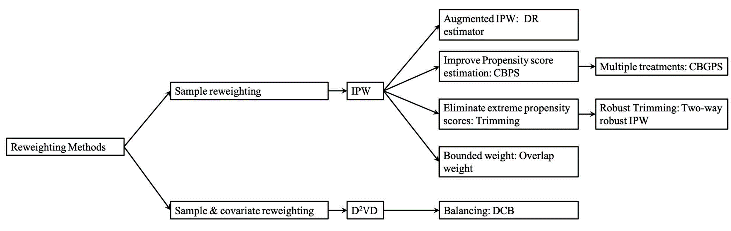
Figure 1. Structure of different re-weighting methods [16].

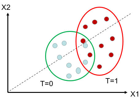
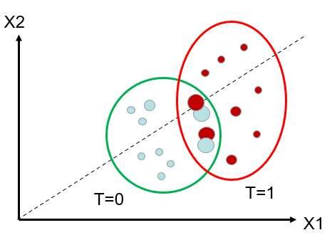
Re-weighting: Figure 2(a) displays the recorded initially data, including the blue-coloured speckles representing the control group and the red-coloured speckles representing the treated group. Notice an area where the confounders X1 and X2 are similar for both treated and untreated units. Figure 2(b) plots the observed data after re-weighting. The red dots (that are on the left side, with lower propensity scores, are assigned a highethanmpared to the original matching. Conversely, the blue dots (that are on the right side, with higher propensity scores, are assigned a higher weicomparedcomparing to the original matching. If there is little overlap between treated and untreated, it signifies that the two groups are very distinct, and we be will not able to extrapolate the effect between them. [15-17]

(a)

(b)

Figure 2. (a) Illustration of the original data. (b) Illustration of the weights of units after re-weighting.

Due to these weaknesses of balancing matching, we adopt the sample re-weighting to eliminate tWe aimr goal is to create a pseudo-population for cases when the distributions of the treated andgroupsrol group are not greatly ifferent, and by assigning the appropriate weight to each unit of samples in the observation dataset. Thmini-batchesi batches are built to imitate the corresponding randomized controlled trial (RCT) process (i.e., the treatment groups are randomly split. Also, the patient distribution in each group is balanced.) Therefore, we can convert an observational study into a pseudo-randomized trial by re-weighting samples, using the propensity score of the treatment they received.

We illustrate the process in Figure 2. Here, before re-weighting the samples, we estimate the propensity scores that represent the conditional probability of receiving the treatment at timestamp \( t+j \) given information up to the current period:

\( {PS_{j}}({\overline{X}_{t}})=P({A_{t+j}}=1|{\overline{X}_{t}},{\overline{A}_{t}},d) for j=1,2,…, ζ \) (2)

Here, \( {A_{t+j}} \) denotes a possible treatment assignment at timestamp \( t+j \) . We use a pre-trained model to calculate the propensity scores for patients in the training set.

Then, we use the inverse propensity score weighting to re-weight the sample and estimate the individual treatment effect as follows:

\( \hat{δ}_{j}^{IPW}=E[\frac{{Y_{t+j}} ∙ {A_{t+j}}}{{PS_{j}}({\overline{X}_{t}})}|{\overline{X}_{t}},{\overline{A}_{t}},d]-E[\frac{{Y_{t+j}} ∙ (1-{A_{t+j}})}{1-{PS_{j}}({\overline{X}_{t}})}|{\overline{X}_{t}},{\overline{A}_{t}},d] \) (3)

Notice that this estimator requires the propensity score to be nonzero (positive), which means that each patient has at least some possibility of receiving and not receiving the treatment. Namely, the treated and control distributions need to be overlapped. This positivity assumption of causal inference is introduced above in Assumption 3.

According to theoretical results, adjusting the scalar propensity score can eliminate bias based on most observed covariates. Yet, IPW's accuracy relies heavily on the accuracy of propensity scores.

4.2. Doubly Robust (DR) or augmented IPW

As described in the previous section, balance matching is not preferred in the study of time-to-treatment observational studies because of its disadvantages: time-consuming and low efficiency. We adopted doubly robust (DR) into our model for debiasing. The doubly robust estimator is also called Augmented IPW (AIPW) since the concept of DR is to combine the inverse propensity score weighting with the outcome regression. [16-21] \( \hat{δ}_{j}^{DR}= E[{\hat{Y}_{t+j}}({A_{t+j}}=1)+\frac{({Y_{t+j}}-{\hat{Y}_{t+j}}({A_{t+j}}=1))∙{A_{t+j}}}{{PS_{j}}({\bar{X}_{t}})}|{\overline{X}_{t}},{\overline{A}_{t}},d] \)

\( -E[{\hat{Y}_{t+j}}({A_{t+j}}=0)+\frac{({Y_{t+j}}-{\hat{Y}_{t+j}}({A_{t+j}}=0))∙{(1-A_{t+j}})}{1-{PS_{j}}({\bar{X}_{t}})}|{\overline{X}_{t}},{\overline{A}_{t}},d] (4) \)

Notice that the DR model consists of two statistical models. In our case, the first is a propensity score model that estimates the probability of receiving antibiotics based on observed covariates. The second model is an outcome regression model that estimates the conditional expectation of the outcome (e.g., survival or recovery) given the treatment and observed covariates.

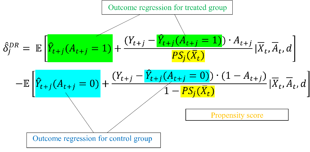
Figure 3. Illustration of combining IPW and outcome regression.

The propensity score calculated by the model and expected to balance the baseline covariates between the time-to-treatment from antibiotics and the control groups in the observational study. Moreover, the propensity scores represent the likelihood of receiving the treatment based on the covariates, such as the severity of syndromes. Then, the algorithm uses the propensity score to balance the distribution of the covariates between the treated and the untreated groups. A doubly robust estimator would be unbiased when the propensity score estimation or the outcome regression is correct.

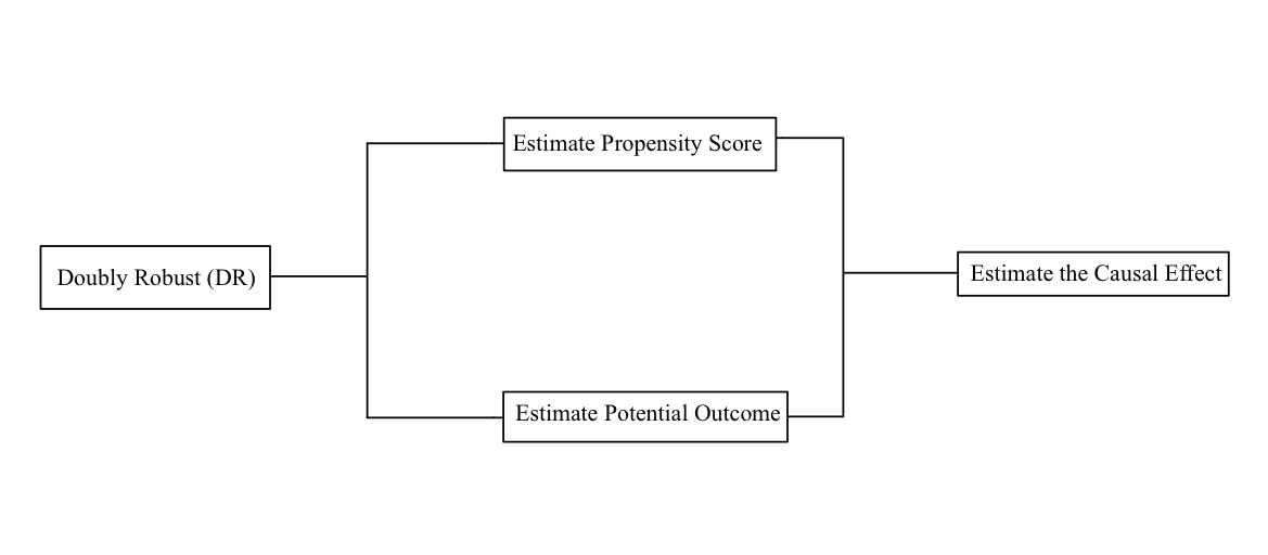
Figure 4. Procedure of Doubly Robust [16].

5. Results

5.1. Model performance

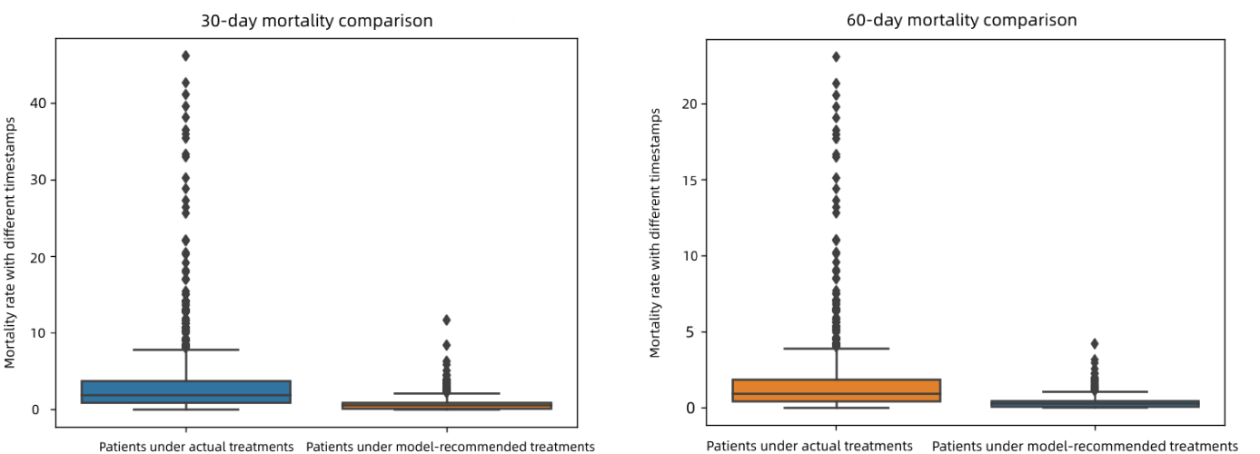
Figure 5. (a) 30-day mortality rate comparison (b) 60-day mortality rate comparison.

As shown in Figures 5(a) and 5(b), we calculated and compared the 30-day and 60-day mortality rates. In Figures 5(a) and 5(b), the left data represents patients taking actual treatments, and the right represents patients taking model-recommended medicines. We found that patients receiving treatment at timestamps that are not recommended had higher average mortality rates. Patients receiving treatment with the identical recommended timestamps had lower overall mortality rates. We evaluated models for different follow-up periods (i.e., \( ζ ∈ \lbrace 1,2,3,…\rbrace \) ). For 60-day mortality rate, there is no significant difference compared to the 30-day mortality rate, with almost the same mortality rate at all timestamps.

Overall, the mortality rate of patients under actual treatments is higher than that of patients under model-recommended treatments. The outcomes indicate that our model recommends effective treatment assignment, as reflected by the mortality rate and estimates when doctors should decide to give antibiotics to patients with sepsis. This proves our model's robustness to be applied to various datasets with distinct characteristic distributions.

5.2. Individual analysis

To explain in detail how our model is based on ITE estimation to recommend antibiotics, we used a real-world patient case and predicted the data as shown in Figure 6:

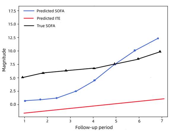
Figure 6. SOFA score and ITE prediction.

As shown in Figure 6, we use the predicted ITEs as the criteria for antibiotic assignment recommendation. To be precise, we recommend antibiotics at each timestamp \( j \) if the ITE is lower than zero \( ({\hat{δ}_{j}} \lt 0) \) , which means the predicted SOFA score for \( T=1 \) is lower than the accurate SOFA score for \( T=0 \) . We will not recommend if the predicted ITE is more significant than zero \( ({\hat{δ}_{j}} \gt 0) \) , where zero is the border that represents no difference between whether to take antibiotics or not \( ({\hat{δ}_{j}}=0) \) .

In the case of a specific patient, illustrated by Figure 6, the predicted ITE is negative for \( 0 \lt j \lt 5 \) in the follow-up period. In contrast, the predicted SOFA values are much lower than the actual SOFA values at the recommended time of antibiotics. Therefore, the optimal treatment recommendation of our model is to take antibiotics before \( j=5 \) and stop the antibiotic after \( j=5 \) . Our model can identify adequate periods of antibiotic assignment for septic patients to relieve their conditions while lowering mortality.

5.3. Case study with variables contribution

The Spearman rank correlation coefficient, \( ρ \) , is the Pearson correlation coefficient between hierarchical variables [22,23], a nonparametric correlation measure based on data ranks. It uses a monotone equation to evaluate the associations between two status variables. The value of the Spearman coefficient lies in the range of +1 to -1 where,

• A perfect association of rank is indicated by a \( ρ \) value of +1.

• Zero association of ranks is indicated by a \( ρ \) value of 0.

• A perfect negative association of class is characterized by a \( ρ \) value of -1.

When the \( ρ \) value is closer to 0, the association between the two levels becomes weaker.

For samples with a size of \( n \) , \( n \) raw data are converted into hierarchical data, with correlation coefficients \( ρ \) by

\( ρ=\frac{\sum _{i}({x_{i}}-\overline{x})({y_{i}}-\overline{y})}{\sqrt[]{\sum _{i}{({x_{i}}-\overline{x})^{2}}\sum _{i}{({y_{i}}-\overline{y})^{2}}}} \) (5)

Therefore, we visualize variable-level contribution in Figure 7. The following heat map is obtained by analyzing the relationship between the above variables. Here, the variables include the vital signs (temperature and respiratory rate) and the lab tests (glucose, potassium, sodium, blood urea nitrogen (BUN), anion gap, and platelet); the static covariates include gender and age.

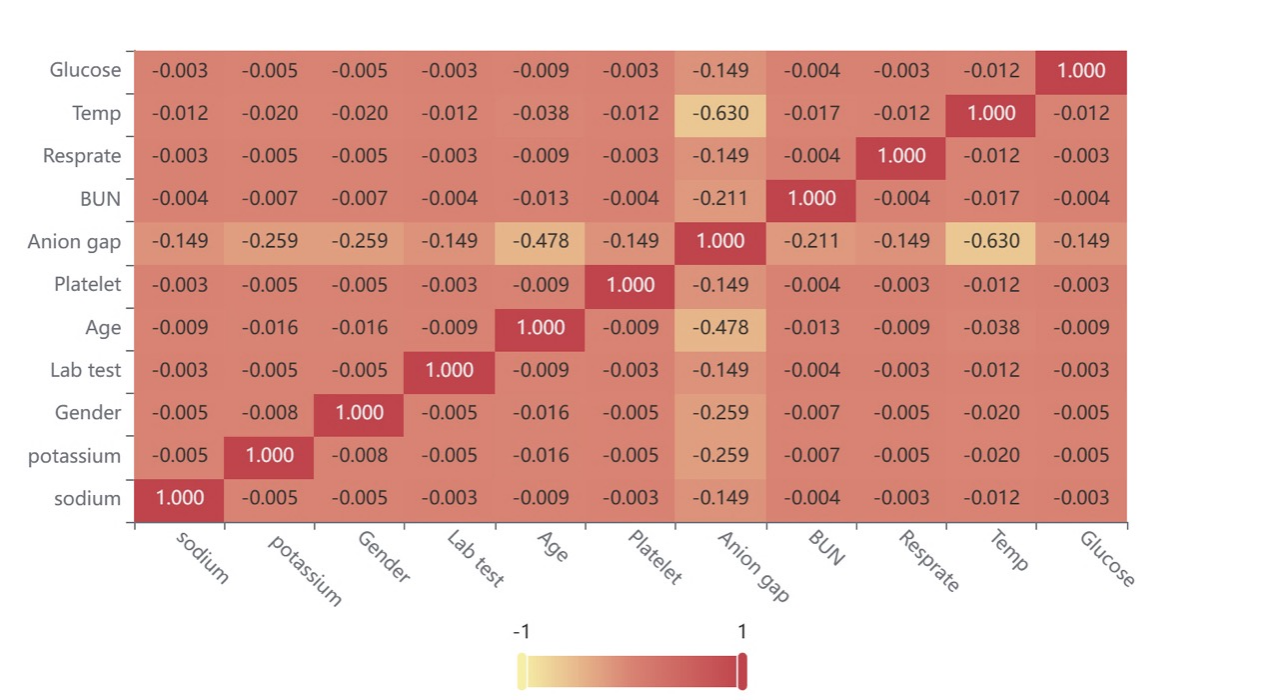
Figure 7. Heat map for the correlation of the variables.

Figure 7 shows the value of the correlation coefficient in the form of a heat map, mainly indicating the size of the matter through color depth. This suggests that the correlation of most variables is weak, while a small number of variables have a specific correlation. Within a controllable range, there is almost no mutual influence between variables, and the research is reliable.

6. Discussion

In this paper, we show how reinforcement learning can solve complicated medical problems and suggest personalized treatment plans for sepsis that doctors can understand. In a different group, patients who got the treatment plan recommended by AI had the lowest death rate.

When a doctor's treatment differs from what AI recommends, the common problem is that too few vasopressor drugs are used. Excessive infusion is also associated with a poor prognosis. Early use of low-dose vasopressors is considered adequate for sepsis. Our research supports these strategies, but more importantly, it allows treatment to be personalized for each patient.

Physicians often need to make subjective clinical judgments about treatment strategies. Nevertheless, computer models can give more information about choosing the best design, like avoiding antibiotic resistance and focusing on long-term survival. The reinforcement learning method we made does not care what kind of data is used so it can be used in any clinical setting with many data and for many medical interventions. With the development of omics technology, AI physicians can add information to improve status definitions and guide more treatment in selected patient groups. Different kinds of information about patients will be fed into the electronic health record software with our algorithm, which will then suggest several ways to help the patient. This system can be utilized in real-time.

However, our research could be improved. Although our dataset is extensive and consists of routinely collected clinical data, some locations and patients must be excluded due to poor quality data records or missing data. Finally, some experimental medical values are not immediately available to clinicians when making decisions but are available to AI.

Medical workers should test in different healthcare settings and make decisions based on real-time clinical cases and data. However, lowering the death rate of septic patients by a small amount could save the lives of thousands of people worldwide every year. In the past 10–15 years, attempts to develop new treatment strategies to reduce mortality from sepsis have been unsuccessful. Using computerized decision-making systems to guide treatment better and improve prognosis is a much-needed method.

7. Conclusion

The primary way for IPW to adjust confounders is to balance confounders at different treatment levels with treatment weight. In our model, we applied a pseudo population to different treatment application trajectories where all measured confounders are balanced between other treatment groups. The obtained data meet the requirements of absolute randomized controlled trials. Therefore, causal inference can be made by comparing groups through t-tests.

Applying stable inverse probability weighted censoring to all models addresses potential selection biases due to missing data and missed visits. Results that can be generalized to the initial target patient are provided. The application of weighting can alleviate the bias caused by this nonrandom selection and deletion so that results with a subset of complete data and follow-up can be generalized to the initial goal. IPW can only handle data loss situations that can be predicted using observed information.

Because of its unique characteristic, the Doubly Robust estimator allows a more rigorous analysis of observational data of the patients by detecting the potential factors that might change the outcomes. However, if the lack of data depends on the future time of the results, which is unobservable, then this dependency can only be captured reliably by making speculative assumptions. Thus, it is best to use stable weights when using IPW since they have less variability and can therefore produce a more efficient estimation.

By running the models, we have proved the hypothesis that by adopting the IPW method and the DR estimator, the recommended time-to-treatment processes can significantly decrease the mortality rate. More specifically, by analyzing both the 30-days and the 60-day mortality comparison graphs we recorded, it is evident that the model has concentrated the margin between patients under model-recommended treatment and those under actual therapy to less than 3%.

Nevertheless, improvements are still required to successfully facilitate the machine learning models and concepts in the practical treatment process of sepsis because there is still an area of progress in our research. With this being stated, multiple excellent causal inference techniques are developed by data scientists and will be tested in the future.

Authors’ contributions

Our group decided on the research topic together. Junde Qian wrote the abstract. Haoxiang Xia and Junde Qian wrote the introduction. Junde Qian and Linwei Ye wrote the preliminary assumptions. For the method section, Junde Qian and Dingrong Xiao are responsible for developing inverse propensity score weighting; Haoxiang Xia is accountable for developing doubly robust. Dingrong Xiao ran the program for the experiments, and Dingrong Xiao and Junde Qian interpreted the results. Dingrong Xiao and Haoxiang Xia wrote the conclusion and discussion. Our group cooperated in the research and wrote the manuscript separately.

Acknowledgement

Dingrong Xiao, Haoxiang Xia and Junde Qian are the contributed equally to this work and should be considered co-first authors.

References

[1]. Septicemia. Septicemia | Johns Hopkins Medicine. (2019, November 19). Retrieved April 2, 2023, from https://www.hopkinsmedicine.org/health/conditions-and-diseases/septicemia
[2]. Weiss, S. L., Peters, M. J., Alhazzani, W., Agus, M. S., Flori, H. R., Inwald, D. P., Nadel, S., Schlapbach, L. J., Tasker, R. C., Argent, A. C., Brierley, J., Carcillo, J., Carrol, E. D., Carroll, C. L., Cheifetz, I. M., Choong, K., Cies, J. J., Cruz, A. T., De Luca, D., … Tissieres, P. (2020). Surviving sepsis campaign international guidelines for the management of septic shock and sepsis-associated organ dysfunction in children. Intensive Care Medicine, 46(S1), 10–67. https://doi.org/10.1007/s00134-019-05878-6
[3]. Martínez, M. L., Plata-Menchaca, E. P., Ruiz-Rodríguez, J. C., & Ferrer, R. (2020). An approach to antibiotic treatment in patients with sepsis. Journal of Thoracic Disease, 12(3), 1007–1021. https://doi.org/10.21037/jtd.2020.01.47
[4]. Im, Y., Kang, D., Ko, R.-E., Lee, Y. J., Lim, S. Y., Park, S., Na, S. J., Chung, C. R., Park, M. H., Oh, D. K., Lim, C.-M., Suh, G. Y., Lim, C.-M., Hong, S.-B., Oh, D. K., Suh, G. Y., Jeon, K., Ko, R.-E., Cho, Y.-J., … Moon, J. Y. (2022). Time-to-antibiotics and clinical outcomes in patients with sepsis and septic shock: A prospective nationwide Multicenter Cohort Study. Critical Care, 26(1). https://doi.org/10.1186/s13054-021-03883-0
[5]. Schuetz, P., Raad, I., & Amin, D. N. (2013). Using procalcitonin-guided algorithms to improve antimicrobial therapy in ICU patients with respiratory infections and sepsis. Current Opinion in Critical Care, 19(5), 453–460. https://doi.org/10.1097/mcc.0b013e328363bd38
[6]. Liu, R., Buck, K. H., Caterino, J. M., & Zhang, P. (2022). Estimating treatment effects for time-to-treatment antibiotic stewardship in sepsis, 1–13. https://doi.org/10.1101/2022.08.29.22279330
[7]. Zhang, D., Micek, S. T., & Kollef, M. H. (2015). Time to appropriate antibiotic therapy is an independent determinant of postinfection ICU and hospital lengths of stay in patients with sepsis*. Critical Care Medicine, 43(10), 2133–2140. https://doi.org/10.1097/ccm.0000000000001140
[8]. Seaman, S. R., & White, I. R. (2011). Review of inverse probability weighting for dealing with missing data. Statistical Methods in Medical Research, 22(3), 278–295. https://doi.org/10.1177/0962280210395740
[9]. Liu, O. L., Liu, H., Roohr, K. C., & McCaffrey, D. F. (2016). Investigating college learning gain: Exploring a propensity score weighting approach. Journal of Educational Measurement, 53(3), 352–367. https://doi.org/10.1111/jedm.12112
[10]. Funk, M. J., Westreich, D., Wiesen, C., Stürmer, T., Brookhart, M. A., & Davidian, M. (2011). Doubly robust estimation of causal effects. American Journal of Epidemiology, 173(7), 761–767. https://doi.org/10.1093/aje/kwq439
[11]. Kennedy, E. H. (2022, May 26). Towards optimal doubly robust estimation of heterogeneous causal effects. arXiv.org. Retrieved March 29, 2023, from https://arxiv.org/abs/2004.14497
[12]. Lambden, S., Laterre, P. F., Levy, M. M., & Francois, B. (2019). The SOFA score—development, utility and challenges of accurate assessment in clinical trials. Critical Care, 23(1). https://doi.org/10.1186/s13054-019-2663-7
[13]. Seymour, C. W., Gesten, F., Prescott, H. C., Friedrich, M. E., Iwashyna, T. J., Phillips, G. S., Lemeshow, S., Osborn, T., Terry, K. M., & Levy, M. M. (2017). Time to treatment and mortality during mandated emergency care for sepsis. New England Journal of Medicine, 376(23), 2235–2244. https://doi.org/10.1056/nejmoa1703058
[14]. Guirgis, F. W., Jones, L., Esma, R., Weiss, A., McCurdy, K., Ferreira, J., Cannon, C., McLauchlin, L., Smotherman, C., Kraemer, D. F., Gerdik, C., Webb, K., Ra, J., Moore, F. A., & Gray-Eurom, K. (2017). Managing sepsis: Electronic recognition, rapid response teams, and Standardized Care Save Lives. Journal of Critical Care, 40, 296–302. https://doi.org/10.1016/j.jcrc.2017.04.005
[15]. Pearl, J., Glymour, M., & Jewell, N. P. (2016). Counterfactuals and Their Applications. In Causal inference in statistics: A Primer (pp. 89–120). essay, Wiley.
[16]. Li, S., Yao, L., Li, Y., Gao, J., & Zhang, A. (2020). Representation learning for causal inference. AAAI-20 Tutorial on Causal Inference. (n.d.). Retrieved March 29, 2023, from https://cobweb.cs.uga.edu/~shengli/AAAI20-Causal-Tutorial.html
[17]. Facure, M. (2022). Causal Inference for The Brave and True [web log]. Retrieved March 28, 2023, from https://matheusfacure.github.io/python-causality-handbook/landing-page.html.
[18]. Sontag, D. (2023). Lecture 11: Causal Inference Part 2. 6.871/HST.956: Machine Learning for Healthcare.
[19]. Künzel, S. R., Sekhon, J. S., Bickel, P. J., & Yu, B. (2019). Metalearners for estimating heterogeneous treatment effects using machine learning. Proceedings of the National Academy of Sciences, 116(10), 4156–4165. https://doi.org/10.1073/pnas.1804597116
[20]. Nie, X., & Wager, S. (2020). Quasi-oracle estimation of heterogeneous treatment effects. Biometrika, 108(2), 299–319. https://doi.org/10.1093/biomet/asaa076
[21]. Jacob, D. (2021). CATE meets ML - conditional average treatment effect and machine learning. SSRN Electronic Journal. https://doi.org/10.2139/ssrn.3816558
[22]. Xiao, C., Ye, J., Esteves, R. M., & Rong, C. (2015). Using Spearman's correlation coefficients for exploratory data analysis on Big Dataset. Concurrency and Computation: Practice and Experience, 28(14), 3866–3878. https://doi.org/10.1002/cpe.3745
[23]. Bhat, A. (2022). Spearman correlation coefficient: Formula + Calculation [web log]. Retrieved April 2, 2023, from https://www.questionpro.com/blog/spearmans-rank-coefficient-of-correlation/.
Cite this article
Xiao,D.;Xia,H.;Qian,J.;Ye,L.;Hu,C. (2023). Applying Inverse Propensity Score Weighting and Doubly Robust for Treatment Effect Estimation in Sepsis. Applied and Computational Engineering,8,835-846.
Data availability
The datasets used and/or analyzed during the current study will be available from the authors upon reasonable request.
Disclaimer/Publisher's Note
The statements, opinions and data contained in all publications are solely those of the individual author(s) and contributor(s) and not of EWA Publishing and/or the editor(s). EWA Publishing and/or the editor(s) disclaim responsibility for any injury to people or property resulting from any ideas, methods, instructions or products referred to in the content.
About volume
Volume title: Proceedings of the 2023 International Conference on Software Engineering and Machine Learning
© 2024 by the author(s). Licensee EWA Publishing, Oxford, UK. This article is an open access article distributed under the terms and
conditions of the Creative Commons Attribution (CC BY) license. Authors who
publish this series agree to the following terms:
1. Authors retain copyright and grant the series right of first publication with the work simultaneously licensed under a Creative Commons
Attribution License that allows others to share the work with an acknowledgment of the work's authorship and initial publication in this
series.
2. Authors are able to enter into separate, additional contractual arrangements for the non-exclusive distribution of the series's published
version of the work (e.g., post it to an institutional repository or publish it in a book), with an acknowledgment of its initial
publication in this series.
3. Authors are permitted and encouraged to post their work online (e.g., in institutional repositories or on their website) prior to and
during the submission process, as it can lead to productive exchanges, as well as earlier and greater citation of published work (See
Open access policy for details).