1. Introduction

1.1. Context and problem background

In many signal chains (such as numerical calibration, filter gain update, coordinate transformation, etc.), division operations are repeatedly used. Directly implementing division operations on an FPGA usually results in large-scale combinational circuits or multi-cycle state machines generated by synthesizers, which have problems such as long critical paths, high wiring pressure, high DSP and LUT usage rates, and difficulty in achieving both high frequency and low latency simultaneously [1]. If support for signed and decimal numbers is added, the control and verification costs will increase rapidly, and the correctness of boundary values and convergence conditions will be more difficult to guarantee. Due to these engineering limitations, we adopted the "first calculate the reciprocal and then multiply" method, which effectively completes division operations by multiplying the dividend by the reciprocal. The reciprocal is generated through Newton-Raphson (NR) iteration and only relies on multiplication and addition, which is naturally suitable for DSP48 multiply-add chains [2], facilitating strong pipelining and register segmentation, and is also convenient for time grouping reuse in resource-constrained scenarios and channel interleaving in high throughput scenarios. Combined with the fixed-point operation mode, the divisor can be standardized to a controllable range first, then an initial value is provided by a small lookup table, and several iterations are carried out; its quadratic convergence characteristic enables the accuracy to increase rapidly with the increase in the number of steps. Common formats such as Q16.16 usually reach the target after only two iterations. For powers of two divisors, a fast path can be used, directly obtaining the result through shifting, thereby combining the general path with special cases optimization to achieve a more stable engineering balance between resources, timing, and throughput.

1.2. Objectives and evaluation metrics

Our goal is to demonstrate an optimized NR frequency divider under fixed conditions, aiming to minimize the usage of digital signal processors (DSPs), while meeting the accuracy requirements of the application, increasing the operating frequency, and limiting the total latency within a predictable number of pipeline stages. With Q16.16 as the core, we combine normalization and small LUT initial values, 2-power pathways, powerful pipelines, and segmented pipelines with multiplication-addition chains. We also provide two configurations, "reuse" and "interleaving", to balance throughput and resource consumption. The evaluation is based on three categories of indicators: in terms of resources, we focus on the number of LUTs, the number of registers, and the number of DSPs; in terms of timing, we focus on critical path margin, end-to-end delay, and per-cycle throughput; in terms of accuracy, we mainly use the maximum and median relative errors of random and boundary samples. At the same time, we record the impact of the size of the initial value table and the number of iteration steps on the error and resources to ensure stable and reliable performance in the actual signal chain.

2. Basic circuit implementation and issues: fundamental circuit modifications

2.1. Baseline circuit implementation and issues

2.1.1. Fundamentals of circuit implementation explained

First, a fundamental explanation of this paper's core subject is required: Newton–Raphson approximate division. The Newton–Raphson iteration method can be employed to compute reciprocals for division. Its fundamental principle involves iteratively approximating the true reciprocal. For division, let the desired reciprocal be 1/d . Taking equation (1) yields the iterative equation (2):

$$ f\left(x\right)=\frac{1}{x} - d$$(1)

$$ x_{n+1}=x_n * (2 - d * x_n)$$(2)

The formula (2) indicates that the next iteration value  $$ {\mathrm{x}}_{\mathrm{n}+1}$$  is obtained by multiplying the current approximation  $$ {\mathrm{x}}_{\mathrm{n}}$$  by the correction factor  $$ (2\mathrm{ }-\mathrm{ }\mathrm{d}\mathrm{ }\mathrm{*}\mathrm{ }{\mathrm{x}}_{\mathrm{n}})$$  . This method exhibits quadratic convergence, and a suitable initial value enables rapid convergence towards 1/d [3].

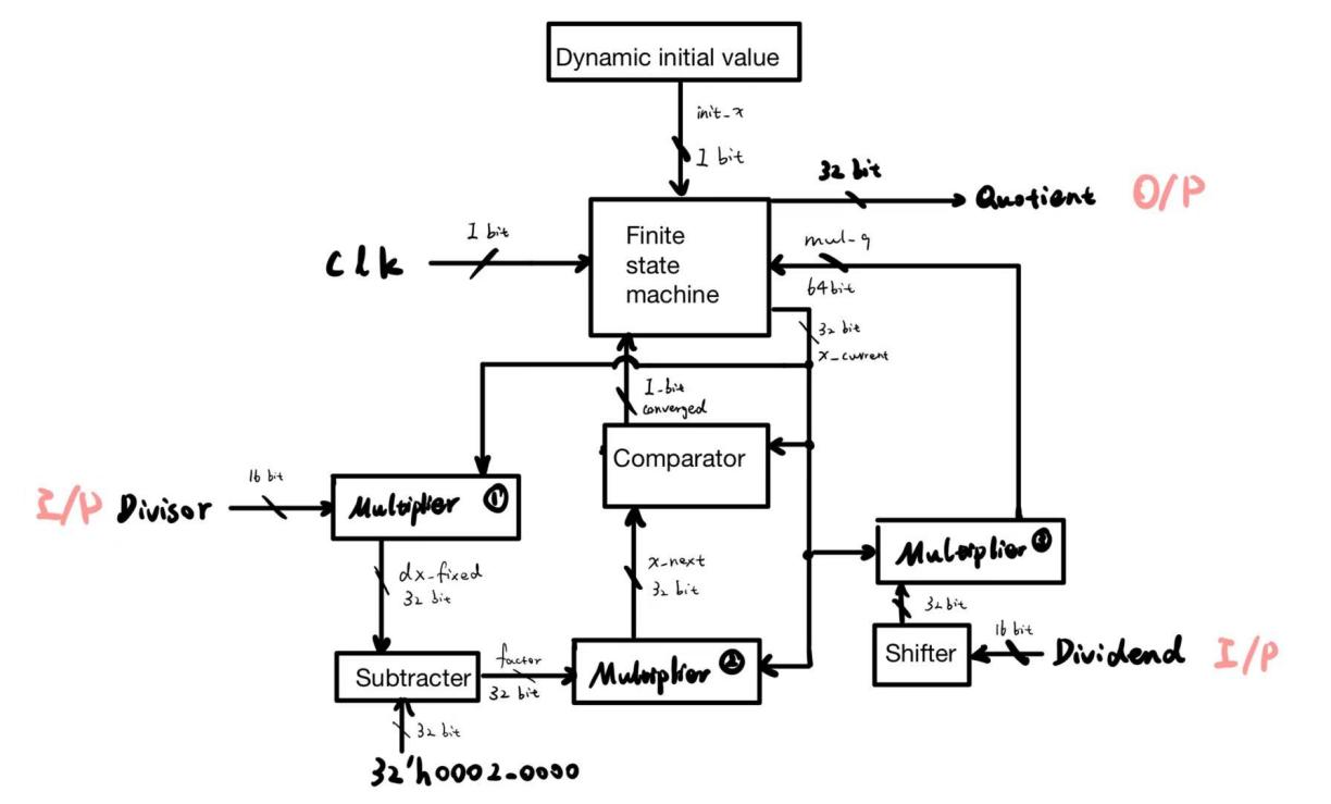
The NewtonDivider module in the provided code performs division according to the aforementioned iterative principle. The circuit employs a 32-bit fixed-point Q16.16 format (16-bit fractional part), where 1.0 is represented as 65536. First, the initial approximation  $$ {\mathrm{x}}_0$$  is computed via the following code:

\begin{lstlisting}[language=Verilog]

wire [31:0] init_x = (divisor != 0) ? (32'd65536 / divisor) : 32'd0;

\end{lstlisting}

Here, 65536 represents the fixed-point number 1.0[4]. When divisor is non-zero, the initialreciprocal estimate is obtained as 65536/divisor. Subsequently, the circuit enters iterativecomputation, performing the following operations in each round:

\begin{lstlisting}[language=Verilog]

wire [31:0] two_fixed = 32'h0002_0000; // 2.0 in Q16.16

assign factor = $signed(two_fixed) - $signed(dx_fixed);

assign mul_tmp = $signed(x_current) * factor;

wire [31:0] x_next = mul_tmp[47:16];

\end{lstlisting}

The above code implements the update equation (2) : first, factor is computed to yield $$ (2\mathrm{ }-\mathrm{ }\mathrm{d}\mathrm{ }\mathrm{*}\mathrm{ }{\mathrm{x}}_{\mathrm{n}})$$ , then the current value x_current is multiplied by factor to produce the new x_next. By truncating the product at positions [47:16] to align the fixed-point multiplication result (preserving 16 decimal places). The updated x_current will be closer to 1/d.

To determine convergence, a threshold is set to compare the difference between consecutive iterations. When  $$ |{\mathrm{x}}_{\mathrm{n}+1}\mathrm{ }-{\mathrm{x}}_{\mathrm{n}}|$$  is less than 0.001, iteration may cease. The corresponding check in the code is as follows:

\begin{lstlisting}[language=Verilog]

localparam THRESH = 32'd66; // 0.001 * 2^16

assign converged = (abs_diff < THRESH);

\end{lstlisting}

When converged is true, it indicates that the iteration satisfies the accuracy requirement. At this point, the FSM exits the loop and proceeds to calculate the final result. The module multiplies the dividend by the last x_current value to obtain the fixed-point representation of the quotient, mul_q, and extracts its upper 32 bits as the output:

\begin{lstlisting}[language=Verilog]

quotient <= mul_q[47:16];

\end{lstlisting}

The entire process is controlled by a finite state machine, encompassing states such as IDLE (awaiting initiation), INIT (loading initial values), CALC_FACTOR/UPDATE_X (iterative computation), CHECK_CONV (verifying convergence), CALC_QUOT (calculating the quotient), and DONE (outputting results), which coordinate the aforementioned operations. Upon triggering the start signal, the FSM cycles through iterative computations until convergence is achieved. It then calculates the final quotient and signals completion via the ready signal.

The Figure 1 is a block diagram of my circuit code logic, which may serve as a reference.

2.1.2. Issues, disadvantages and potential risks in the initial code

The initial baseline implementation had multiple issues. The FSM control process design is unreasonable. My initial version did not adopt a concise iteration counting mechanism, and the state machine design was complex (executing multiple operations in a single state). The control logic makes it difficult to understand and not conducive to subsequent expansion. The initial value selection of the iterative algorithm is incorrect. The baseline implementation obtains an initial reciprocal approximation through hard coded division (such as directly calculating x0=1.0/divisor), which not only consumes additional resources but also deviates from the original intention of the Newton Raphson algorithm to avoid direct division. If fixed initial values are used, there will be a lack of adaptability to different inputs, which can lead to slow convergence or even divergence in some cases. At the same time, this design only supports integer input/output interfaces, and the input is treated as a pure integer (with a decimal part of 0), which cannot directly generate non integer quotient and limits its application scope. Finally, the definition of termination conditions for iteration is insufficient. The dynamic error evaluation mechanism used in the benchmark version is not robust enough, resulting in unreliable convergence criteria. This may lead to premature termination or insufficient accuracy, and it cannot be guaranteed that accuracy requirements will be met under all conditions. For example, if there is a significant deviation between the previous iteration value and the correct value, even if the difference between the subsequent iteration value and the previous iteration value is minimal, the result will still be distorted. Thus, these defects result in significant disadvantages for the benchmark circuit in terms of control capability, accuracy performance, and flexibility.

2.2. Circuit modification (feasible implementation improvements)

Initially, I broke down the Newton iteration method into several steps and adopted the FSM (Initialization, Calculate Factor, Update x, Check Convergence, Output) logic. This logic was clear and straightforward, but there were too many states, resulting in a bloated control part [5]. Later, I transformed it into a "rhythm counter" process: add an iteration counter, start it, and increment it in a fixed sequence in each clock cycle; when the convergence condition is met or the iteration limit is reached, exit. In this way, there is no need to maintain a bunch of intermediate states (such as CALC_FACTOR/UPDATE_X/CHECK_CONV), and the design, verification, and scalability of the control unit can be improved significantly [6].

Decimal support is achieved through fixed-point arithmetic. First, scale the input value to the target precision (for example, if two decimal places are required, multiply by 100 and round to the nearest integer), and then send it as a 16-bit unsigned value; internally, it is uniformly represented as Q16.16 (16-bit integer + 16-bit fraction), and the result is output in this format. For example, (7.00 ÷ 2.30) becomes (700 ÷ 230), and the result can be accurately represented in a fixed form. Without using floating-point numbers, it can cover more scenarios in a fixed decimal form and is more practical.

\begin{lstlisting}[language=Verilog]

module NewtonDivider(

...

input wire [15:0] dividend, // Dividend (supports two decimal places; e.g., 7.00 should be entered as 700)

input wire [15:0] divisor, // Divisor (supports two decimal places; e.g., 2.30 should be entered as 230)

...

);

\end{lstlisting}

The annotation in the aforementioned port definition indicates support for fractional values: both input and output are processed in the agreed fixed-point format with two decimal places. Through this scaled representation, the circuit maintains fractional precision while enabling internal operations to utilise integer logic, thereby avoiding the complexity of floating-point calculations [7].

Then, in order to accelerate the convergence of Newton's iteration, I redesigned and improved the method for obtaining the initial reciprocal value  $$ {\mathrm{x}}_0$$[8]. I used the rough lookup table (LUT) method to approximately replace the precise calculation. The old version directly provided a fixed initial value obtained through division, or I also tried using a simple constant. Now, based on the size of the divisor, a closer initial estimate is dynamically selected. I roughly estimated the reciprocal by detecting the binary amplitude (the position of the most significant bit) of the divisor. For example, in the circuit, the logic for calculating the highest significant bit (msb_index) of the divisor was added, and based on it, the initial  $$ {\mathrm{x}}_0$$  was selected:

\begin{lstlisting}[language=Verilog]

// Calculate the most significant bit of the divisor msb_index

always @(*) begin

if (divisor >= 16'h8000) msb_index = 15;

else if (divisor >= 16'h4000) msb_index = 14;

... // (Further similar determinations omitted)

else if (divisor >= 16'h0002) msb_index = 1;

else msb_index = 0;

end

// Determine whether the divisor is a power of 2, and compute the initial reciprocal estimate value init_x

wire power_of_two = (divisor != 0) && ((divisor & (divisor - 1)) == 0);

wire [31:0] init_x = (divisor != 0) ?

(32'd1 << (power_of_two ? (16 - msb_index) : (15 - msb_index))): 32'd0;

\end{lstlisting}

The above code is equivalent to a small LUT (Look-Up Table). It selects different initial values of  $$ {\mathrm{x}}_0$$  based on the range of the divisor. When the divisor is exactly a power of 2, its reciprocal is precisely the corresponding negative power of 2, and the circuit directly shifts left by 1 to obtain the exact reciprocal (for example, if the divisor is  $$ 2^{\mathrm{k}}$$ , then the initial  $$ {\mathrm{x}}_0\mathrm{ }=\mathrm{ }{2}^{-\mathrm{k}}$$  is achieved in Q16.16 format through 1 << (16-k)); if the divisor is not a power of 2, an estimated value slightly less than the true reciprocal is taken (using 1 << (15 - msb_index), which is one bit less than the exact value), ensuring that the initial estimate is not too large. The reason for this processing is that in the Newton method, a smaller initial value usually ensures stable convergence of the iteration. Using a rough LUT initial value can avoid directly performing division operations, and the hardware cost is very low (only some comparisons and shift logic are needed), but it can significantly accelerate the convergence of the iteration: a good initial value can reach the required accuracy in fewer iteration steps.

Next, I will explain the rounding strategy I used. In the design, the Q16.16 fixed-point format was adopted to uniformly represent the real numbers during the iterative process. It includes both the integer part and the fractional part. The integer bit width of the Q16.16 representation is 16 bits, and the fractional bit width is also 16 bits. Therefore, the values are represented in 32-bit fixed-point format in the hardware. For example, the constant 2 is represented as 0x0002_0000 in the Q16.16 format. Fixed-point multiplication produces a result with double the bit width, so after each multiplication, it needs to be aligned to the fixed-point bit width, usually by discarding the low 16 bits to achieve the equivalent of dividing by  $$ 2^{16}$$  scaling. This point is reflected in the code multiple times, such as taking the high-order part after calculating the product as the result:

\begin{lstlisting}[language=Verilog]

wire [31:0] two_fixed = 32'h0002_0000; // The constant 2 represented as Q16.16

// Calculate d * x_n and align to Q16.16 format

assign mul_dx = $signed({1'b0, divisor, 16'b0}) * $signed(x_current);

wire [31:0] dx_fixed = mul_dx[47:16]; // Shift the product right by 16 bits, aligning to Q16.16

// Calculate Newton's iteration factor: factor = 2 - d * x_n

assign factor = $signed(two_fixed) - $signed(dx_fixed);

// Update iteration value: x_{n+1} = x_n * factor (result aligned to Q16.16)

assign mul_tmp = $signed(x_current) * $signed(factor);

wire [31:0] x_next = mul_tmp[47:16]; // Shift the product right by 16 bits to obtain the result Q16.16

...

localparam THRESH = 32'd66; // Convergence threshold ≈ 0.001 (as per Q16.16)

...

// Final quotient calculation: quotient = dividend * x_current (result right-shifted 16 bits for alignment)

assign mul_q = $signed({1'b0, dividend, 16'b0}) * $signed(x_current);

...

quotient <= mul_q[47:16];

\end{lstlisting}

As mentioned above, after each multiplication operation, the lowest 16 decimal digits of the result are truncated to [47:16] bits, ensuring that the result remains in the Q16.16 format. Although truncation introduces a certain degree of error deviation, the convergence process of the Newton iteration can tolerate and gradually reduce this error. This design also sets a convergence threshold THRESH = 66 (approximately 0.001 in Q16.16 format) to determine when the iteration should stop. When the difference between two consecutive iterations is lower than this threshold, the result is considered to be accurate enough (thereafter, I abandoned this method and instead adopted a fixed number of iterations and conducted convergence evaluation during simulation). In the calculation of the final quotient, the lowest 16 digits are truncated according to the fixed-point format, keeping the quotient in Q16.16 precision. Therefore, the unified fixed-point format combined with a simple and effective rounding and truncation strategy ensures the stability and accuracy of the circuit calculation, while controlling the complexity of the hardware implementation.

3. Throughput and resource optimization

3.1. Reuse of the multiplier module

During the iterative process of the Newton-Raphson divider, multiple 32×32-bit multiplication operations need to be executed. If a separate multiplication module is instantiated for each operation, it will consume a large amount of DSP resources in the FPGA. Therefore, we adopt a strategy of reusing the multiplication module: only one 32×32-bit multiplication unit is instantiated in the hardware design, and the same unit is called cyclically at different operation stages to complete all multiplication calculations. In other words, one multiplication module is time-division multiplexed to calculate intermediate products such as mul_dx, mul_tmp, and mul_q_next in sequence. The following code snippet shows the instantiation method of the multiplication module:

\begin{lstlisting}[language=Verilog]

Multiplier32x32 mult_dx_inst (

.a({abs_div, 16'b0}),

.b(x_current),

.y(mul_dx)

);

\end{lstlisting}

Through such a module reuse design, multiple multipliers that originally needed to be deployed in parallel share the same set of hardware, achieving repeated utilization of the DSP multiplier unit and significantly reducing resource consumption. A 32×32 multiplication operation is typically mapped onto several FPGA DSP Slices; if three parallel multipliers are directly used, DSP consumption will increase exponentially, while reusing a single multiplier hardware significantly reduces DSP usage. In this design, the cost of reusing the multiplier module is that each multiplication operation needs to be executed in a staggered sequence in time and cannot be completed simultaneously in parallel. This will slightly increase the execution delay of the algorithm. However, by introducing pipelining and interleaved parallelism in the subsequent design (see Section C), the potential impact of reduced throughput is minimized. Overall, the reuse of the multiplier module is highly effective in saving hardware resources, at the cost of only a slightly increased complexity in timing scheduling, in exchange for a significant reduction in DSP resource usage [9].

3.2. Multiplexer modification

The design of the multiplier module has been further improved and explored, mainly covering two aspects: (a) attempts to implement fast multiplication based on the Karatsuba algorithm, and (b) the development of a custom multiplier based on shift-add method along with "rounding" approximation processing.

3.2.1. Discussion and trade-offs of Karatsuba algorithm principles

Karatsuba is a well-known fast multiplication algorithm. Its basic idea is to split the large-width multiplication into smaller segments for calculation. Specifically, it divides the two numbers to be multiplied into high-order and low-order parts, and then uses three smaller-scale multiplication operations and several addition and subtraction operations to calculate the original product. Compared with the 4 sub-multiplications required by the ordinary splitting method, Karatsuba ingeniously utilizes the following identity transformation to reduce one multiplication:

Let the high-order product be equation (3) and the low-order product be equation (4); then the cross-product from equation (5) can be rewritten as equation (6), thereby converting the original two multiplications into a single multiplication plus or minus operation [10].

$$ z_2=x_H* y_H$$(3)

$$ z_0=x_L* y_L$$(4)

$$ z_1=x_H* y_L+x_L* y_H$$(5)

$$ z_1=(x_H+ x_L)*(y_L+ y_H) - z_2 - z_0$$(6)

Karatsuba used divide-and-conquer to split a 32×32 multiplication into three 16×16 multiplications, and then combined them through shifting and addition. Theoretically, this method can reduce the complexity of large number multiplication. However, in the 32-bit fixed-point implementation on FPGA, we did not adopt it. There are two reasons for this. Firstly, the hardware needs to manage the alignment, summation, and subtraction of multiple partial products, as well as retain wider intermediate bits, which leads to an increase in overhead and complexity. If the lower bits are truncated, the precision will be insufficient and it will be difficult to meet the requirements of iterative division. Secondly, at the 32-bit scale, the DSP core is already very efficient. Karatsuba often does not reduce the DSP (it still requires three 16×16 multiplications), but instead increases the adder. Considering the implementation difficulty, resource gain, and precision risk, its theoretical advantages cannot be transformed into actual improvements. In fact, it may even have the opposite effect.

3.2.2. Shifted adder and rounding approximation

For the standard multiplier structure, we also explored a custom 32-bit multiplier based on the shift-add principle, and implemented an approximation strategy for rounding the lower bits of the result on this basis. The "shift adder" refers to using the basic principle of binary multiplication: by performing bitwise AND operations between the digits of the multiplicand and the multiplicand to generate partial products, and then performing appropriate shift and addition to obtain the product result [11]. This method is equivalent to manually assembling a multiplier in hardware. The following is a core code snippet of this multiplier module:

\begin{lstlisting}[language=Verilog]

// add and shift

for (i = 0; i < 32; i = i + 1) begin

for (j = 0; j < 32; j = j + 1) begin

if (a[i] & b[j] & ((i + j) >= K)) begin

acc = acc + (64'd1 << (i + j));

end

end

end

// Add a bias to implement rounding functionality

acc = acc + BIAS;

y = acc & ~((64'd1 << K) - 1);

\end{lstlisting}

The above code implements a 32×32 fixed-point multiplication. Here, the parameter K is used to specify the number of low-order bits to be truncated, and the accumulator acc is used to accumulate all valid partial products. The double loop traverses each bit of the multiplier a and the multiplicand b. When the corresponding bit is 1 and the weight of its product bit is not less than the truncation threshold K,  $$ 2^{\mathrm{i}+\mathrm{j}}$$  is added to the accumulator. This effectively amounts to only accumulating the valid parts of the product that are above the lowest K bits, thereby ignoring the contribution of the lowest K bits. Next, the code adds a bias constant equation (7), and then clears the lowest K bits of the accumulator. This bias-clearing operation implements an "approximation by rounding" for the ignored parts: the bias is equivalent to adding 0.5 units before truncation, and after truncation, it is equivalent to rounding the lowest K bits to the nearest integer.

$$ BIAS = 1 << (K-1)$$(7)

This shift-add-multiply unit essentially constructs multiplication within the logic unit, thereby enabling flexible control over the product's precision. By choosing the truncation bit number K, we can balance the computational accuracy and hardware overhead: omitting some lower-order calculations will reduce the occupation of some hardware resources, and rounding off reduces the error introduction. Compared to the built-in DSP multiplication unit in FPGA, this solution is a "lightweight" implementation, suitable as a reference design for evaluating the impact of precision loss. In our project, we wrote the above shift-add-multiply unit for testing the influence of low K-value truncation on the final quotient's precision. The results show that a slight truncation and rounding processing result in a very limited decrease in the quotient's precision, but if too many bits are truncated, the error significantly increases. Therefore, this method can be used as an alternative with adjustable precision or for approximate division implementation in resource-constrained situations. However, it should be noted that the delay of shift-add-multiplication is relatively long (the expansion of the double loop may become a long serial chain on the hardware), so its speed is not as fast as the DSP core multiplication unit for high-performance requirements. Moreover, as the truncation bit number increases, the precision loss may affect the convergence and correctness of the Newton-Raphson iteration. Therefore, in the final implementation, we use this scheme as an evaluation means to balance the trade-offs, and it has not completely replaced the standard multiplier.

3.3. Interleaving dual/quad channel design and application of pipeline technology

To address the potential reduction in throughput rate caused by the reuse of the aforementioned multiplier module, we introduced a design that combines time interleaving (Interleaving) [12], multi-channel parallelism, and deep pipeline in the circuit. Specifically, this design adopts a four-channel time interleaving architecture, dividing the iterative calculation process into 4 pipeline stages, and using registers in the hardware to sequentially transfer the results of each stage, thereby significantly reducing the combinational logic delay of a single stage. In the code, the four-stage pipeline processing is implemented through the pipeline_phase state and a series of registers, and the key segments are as follows:

\begin{lstlisting}[language=Verilog]

case (pipeline_phase)

2'd0: begin

// Stage 0: Store the first multiplication result

mul_dx_reg <= mul_dx;

dx_fixed_reg <= mul_dx[47:16];

end

2'd1: begin

// Stage 1: Calculate the factor

factor_reg <= two_fixed + (~dx_fixed_reg + 1);

end

2'd2: begin

// Stage 2: Store the second multiplication result

mul_tmp_reg <= mul_tmp;

end

2'd3: begin

// Stage 3: Extract x_next, store the third multiplication and update the state

x_next_reg <= mul_tmp_reg[47:16];

mul_q_next_reg <= mul_q_next;

x_current <= x_next_reg;

iter_cnt <= iter_cnt + 1;

...

end

endcase

pipeline_phase <= pipeline_phase + 2'd1;

\end{lstlisting}

The above code clearly demonstrates the application of the four-stage pipeline in iterative operations: The entire Newton iterative process is divided into four stages - 0, 1, 2, and 3. Each stage performs a part of the calculation, and the intermediate results are temporarily stored in registers (such as mul_dx_reg, factor_reg, mul_tmp_reg, x_next_reg, etc.). The direct benefit of this approach is to shorten the critical path: All the calculations that originally needed to be completed within one clock cycle are distributed over four cycles, with each cycle performing only a small part of the calculation. This ensures a significant reduction in the combinational logic level. As a result, the clock frequency limit is increased, and the circuit can run faster. In fact, after the implementation of the four-stage pipeline, our multiplier module can operate stably at a higher main frequency, increasing the number of iterative steps per second.

However, merely having a pipeline alone cannot increase the throughput rate; if each division operation still requires 4 cycles to complete all stages, the output rate of a single result is only 1/4 of the original. Therefore, we utilize the idea of multi-channel interleaved parallelism to fully leverage the parallel processing capability of the pipeline. The term "dual/four-channel interleaving" refers to simultaneously processing different stages of multiple division operations, forming a "flow operation". In the case of a dual-channel setup, the first input can execute stages 0-3 in odd-numbered cycles, and the second input can execute them out of phase in even-numbered cycles. This way, the two inputs alternate occupying the pipeline, each still requiring 4 cycles to complete but with results being produced every 2 cycles overall. Further expanding to a four-channel interleaving, that is, using each segment of the four-stage pipeline to simultaneously handle the different stages of 4 different division tasks: when the first division is at stage 0, the second division is at stage 1, the third at stage 2, and the fourth at stage 3. Thus, with each clock cycle, the pipeline completes one stage of calculation and advances, and when the pipeline is filled, an ideal throughput rate of outputting one result per clock cycle can be achieved. In summary, the four-channel time interleaving enables although each individual operation still requires 4 cycles to complete, it can concurrently produce partial results of 4 different operations within 4 cycles, starting to output new results every 2 cycles from the 5th cycle. This ensures that while resources are reused, the overall throughput of the system does not decrease [13].

In the actual code we designed, since a single division operation needs to complete all iterations before outputting the final quotient value, we mainly utilized the pipeline to improve the performance of a single operation. However, this approach is also applicable to scenarios where multiple division requests are processed in parallel: by simply duplicating an appropriate number of registers and control logic, dual-channel or even quad-channel interleaved execution can be achieved on the hardware. It is worth noting that multi-channel interleaving increases the complexity and resource overhead of the circuit (for example, separate register groups need to be maintained for different channels), but compared to directly adding independent computing units, the increase in resources is small, yet it achieves a nearly linear improvement in throughput [14].

Overall, the adoption of a four-stage pipeline combined with an interleaved multi-channel design brings the following advantages: the critical path becomes shorter, the circuit can operate at a higher frequency, the throughput rate increases/remains unchanged, and more division operations can be completed within a unit of time. However, the main cost is that the output delay increases to a certain extent (for example, a four-stage pipeline requires several cycles to "fill" the pipeline) and the control logic becomes slightly more complex. But overall, this is a very efficient performance optimization method. Through this approach, we successfully designed the divider while ensuring resource control, maintaining a high throughput rate and significantly increasing the clock speed, achieving the goal of optimizing performance.

4. Initial value estimation

4.1. LUT design: high-indexing, table structure and implementation

To accelerate the convergence of the Newton iteration for finding the reciprocal, we used a lookup table (LUT) in the hardware to provide an initial value estimate [15]. Specifically, the magnitude of the divisor is determined based on its most significant bit (msb), which makes the initial estimate interpretable: we know roughly which power of 2 the divisor is located within. In the code, the msb_index is calculated by prioritizing the judgment of the absolute value of abs_div, which is equivalent to finding the index of the highest bit that is 1. As shown in the following code snippet, we successively compare abs_div with the threshold of the descending power to determine its range interval (for example, if abs_div is greater than or equal to 0x8000, the highest bit index is 15, and so on) [16]:

\begin{lstlisting}[language=Verilog]

if (abs_div >= 16'h8000) msb_index = 15;

else if (abs_div >= 16'h4000) msb_index = 14;

......

else if (abs_div >= 16'h0004) msb_index = 2;

else if (abs_div >= 16'h0002) msb_index = 1;

else msb_index = 0;

\end{lstlisting}

After obtaining the msb_index of the divisor through the above logic, we normalize the divisor (by shifting it to the left, aligning its highest bit to a fixed position), and take several bits from the normalized high part as the index for the lookup table. This allows us to select the appropriate reciprocal initial value based on the range where the divisor lies, and the structure is quite intuitive: The LUT divides the possible range of divisor values into multiple sub-intervals based on the high bits. In our design, a 4-bit LUT index is used, dividing the normalized divisor into 16 sub-intervals, and each interval is pre-stored in the LUT with an approximate reciprocal value of the typical point of that interval. The following code example shows the index calculation and table structure of the LUT: First, take the high 4 bits of the normalized divisor norm_div as lut_idx, and then use the case statement to select the corresponding lut_recip value. There are 16 items in the table, covering the possible range of divisor values, and each item is a fixed-point number form of the initial approximate reciprocal value:

\begin{lstlisting}[language=Verilog]

wire [3:0] lut_idx = norm_div[15:12];

case (lut_idx)

4'h0: lut_recip = 32'h000F_083E;

4'h1: lut_recip = 32'h000E_A0F;

......

4'hF: lut_recip = 32'h0008_0208;

endcase

\end{lstlisting}

It can be seen that this lookup table covers 16 sub-intervals within the range of normalized divisors from 0.1000...b to 0.1111...b (in binary). For each interval, an approximate reciprocal value is selected. For example, when lut_idx = 0 (when the normalized divisor is close to 1.0 in the highest interval), the lookup table gives an initial reciprocal value of 0x000F_83E; while when lut_idx = F (when the normalized divisor is the smallest, that is, close to 0.5), it gives a relatively large initial reciprocal value of 0x0008_208. Through this LUT based on the high-order index, we have implemented piecewise approximation of reciprocals in hardware: it intuitively segments according to the size of the divisor, and each segment has a clear initial reciprocal estimate, making the process of selecting the initial value interpretable (able to explain the divisor range corresponding to each LUT constant). This initial estimate init_x either takes the above LUT value shifted by msb_index bits (scaled according to the divisor size), or takes a fast path in special cases where the divisor is a power of 2 or 0. Overall, partly relying on the more accurate initial values provided by the lookup table, the subsequent Newton iteration converges faster, laying the foundation for improving throughput.

4.2. Trade-off between initial estimation accuracy and iteration count

The convergence speed of the Newton-Raphson method depends on the accuracy of the initial estimate. The closer the initial value is to the true reciprocal, the fewer the number of required iterations. This principle is reflected in our design by adjusting the precision of the LUT: the more bits the LUT uses (the finer the segments), the more accurate the initial reciprocal provided, and thus the number of iterations can be reduced. If the size of the LUT is reduced, the initial value is less precise and more iterations are needed to achieve the same level of accuracy. This is a typical trade-off between throughput and resources [17].

For example, for a 16-item LUT with 4-bit indices, only 5 iterations are needed to meet the accuracy requirements. However, if the LUT precision is reduced, for instance, by using a 2-bit index (corresponding to 4 initial value ranges), the initial estimation error increases, and in our implementation, we need to increase the upper limit of the iteration count to ensure accuracy convergence. In the code of the 4 initial value schemes, MAX_ITER is set to 8, which means a maximum of 8 iterations are allowed. This precisely reflects the trade-off between the accuracy of the initial value and the iteration cost. Now, let's further look at the differences in the selection of initial values between these two schemes.

In the scenario with only 4 initial estimates, we divide the divisor range into four segments and select a fixed proportion coefficient for each segment as the initial reciprocal approximation. For example, the interval is divided into [2^k, 1.25·2^k), [1.25·2^k, 1.5·2^k), [1.5·2^k, 1.75·2^k), [1.75·2^k, 2^k), corresponding to the estimated values c0, c1, c2, c3. In the code implementation, first calculate the base value base (the ideal reciprocal value when the divisor is exactly 2^k), and then predefine several coefficients to approximate the reciprocals of different intervals, such as 0.8, 0.67, 0.5714, etc. Proportions. Based on which interval the divisor falls, select the corresponding c value as the initial reciprocal init_x. The following code snippet shows the implementation of the 4 segments of the initial estimation scheme:

\begin{lstlisting}[language=Verilog]

// Initial estimate: 4-bit precision division

wire [31:0] base = 32'h0001_0000 >> msb_index;

// Quadrant intervals (2^k, 1.25·2^k, 1.5·2^k, 1.75·2^k)

wire [15:0] t1 = (16'd1 << msb_index) + (16'd1 << (msb_index - 2));

wire [15:0] t2 = (16'd1 << msb_index) + (16'd2 << (msb_index - 2));

wire [15:0] t3 = (16'd1 << msb_index) + (16'd3 << (msb_index - 2));

wire [31:0] c0 = base;

wire [31:0] c1 = (base * 32'h0000_CCCC) >> 16;

wire [31:0] c2 = (base * 32'h0000_ABAB) >> 16;

wire [31:0] c3 = (base * 32'h0000_9249) >> 16;

wire [31:0] init_x = (abs_div == 0) ? 32'd0 :

(power_of_two) ? base :

(abs_div < t1) ? c0 :

(abs_div < t2) ? c1 :

(abs_div < t3) ? c2 : c3;

\end{lstlisting}

From the above code, it can be seen that the low-precision LUT scheme only selects one of the few pre-estimated values (c0 - c3) based on the interval where the divisor is located. Compared with the fine-grained lookup of the 16-item LUT, this method has lower hardware overhead, but the initial value error is larger and requires more iterations to correct the error. Conversely, when using the 16-item LUT, the initial values for each interval are closer to the true reciprocal, with smaller errors. The Newton iteration only requires a few steps to achieve high precision. Therefore, we set the upper limit of the iteration to 5.

This difference directly affects the throughput performance: In our pipeline implementation, each iteration requires a fixed number of clock cycles (for example, completing one iteration of multiplication and update through four stages of pipeline_phase takes one iteration). As the number of iterations increases, the total number of clock cycles required to complete a division operation also increases accordingly. Taking this design as an example, the 5-iteration scheme requires approximately 20 (5×4 = 20) clock cycles for each division, while the 8-iteration scheme requires 32 clock cycles. The gap is significant. If computationally intensive applications require higher division throughput, we tend to use more accurate initial LUTs to reduce iterations. However, at the same time, larger LUTs (such as 16-entry tables) also mean an increase in resource usage (requiring more constants to be stored or more complex combinational logic). Fortunately, in this design, the 16×32-bit lookup table overhead is very small, and it can be exchanged for a significant reduction in the number of iterations by using a small amount of logic resources.

In conclusion, we made a compromise choice in terms of throughput and resource optimization: by moderately increasing the precision of the lookup table to reduce the number of iterations, and by slightly increasing the hardware resources to achieve performance improvement [18]. We selected the 4-bit LUT index (16 entries) scheme, enabling the system to reach the required accuracy in only 5 iterations, achieving a high division operation throughput rate, while the resource overhead remained within an acceptable range. In contrast, if a smaller LUT was used, although a little storage of the lookup table was saved, the number of iterations increased to 8, and the unit operation delay and total resource consumption might actually increase (more registers and arithmetic units operating repeatedly). Therefore, this design optimizes the initial estimation by increasing the bit width of the LUT, achieving a balance between hardware resources and computation delay, and thus achieving a win-win situation in terms of throughput and resource efficiency.

5. Analysis and implementation of the goldschmidt division algorithm

After completing the study of the Newton-Raphson algorithm, I also investigated new algorithms that can be used as the core principle for constructing a divider. The Goldschmidt algorithm also converts division into a multiplication problem. Its idea is to make the divisor approach 1 through iterative multiplications, and make the dividend converge to the quotient. First, the initial reciprocal approximation x0 is calculated based on the most significant bit (msb) of the divisor (for example, init_x = 1<<(16-msb) to obtain the 1/d estimation in Q16.16 format), then the correction factor  $$ g$$  from equation (8) is iteratively calculated and equation (9) is updated. After the iteration, d approaches 1, and at this point, n is the quotient [19].

$$ g=2 - d_i$$(8)

$$ \{\begin{array}{c}{d}_{i+1}=d_i * g\\ n_{i+1}=n_i * g\end{array}$$(9)

In terms of code implementation, the module first takes the absolute values of the dividend and the divisor, identifies the most significant bit (MSB) of the divisor, and calculates the initial approximate reciprocal x0:

\begin{lstlisting}[language=Verilog]

wire [31:0] init_x = (abs_d != 0) ? (32'd1 << (16 - msb)) : 32'd0;

x0 <= init_x;

\end{lstlisting}

The above code generates the 1/d initial value x0 in the Q16.16 format based on the most significant bit. In the iterative stage, at each step, d_val and n_val (obtained through the pipeline) are first calculated, then the correction factor g_val is computed, and the next-level approximation is updated through parallel multiplication:

\begin{lstlisting}[language=Verilog]

d_val <= pipe_d[47:16];

n_val <= pipe_n[47:16];

g_val <= TWO - pipe_d[47:16];

\end{lstlisting}

In each iteration here, only one subtraction and two parallel multiplications are performed, which enables the algorithm to converge quickly.

In contrast, the Goldschmidt algorithm requires two parallel multipliers for each iteration, although it is fast, the hardware resource consumption is relatively high. While the Newton-Raphson iterative method only needs one multiplier to approximate 1/d, the hardware structure is simpler. Therefore, in this design, the Newton-Raphson iterative method is ultimately adopted to replace the Goldschmidt algorithm in order to reduce the hardware complexity and resource consumption [20].

6. Comparison and summary

Compared to the baseline version, the optimized Newton-Raphson divider (implemented in Verilog) has undergone multiple improvements in both structure and functionality. Firstly, the finite state machine (FSM) structure has been replaced by a clearer counter adding pipeline combination, making the timing and convergence process easier to analyze; the symbol processing has been changed from implicit to explicit, making the symbol boundaries clearer. Secondly, the lookup table (LUT) approximation method is used to replace the initial guess value calculation for division, improving the reliability. Additionally, by eliminating the non-structured termination judgment and introducing a fixed number of iterations, the verification process has been simplified and is more conducive to pipeline implementation. Finally, it supports the conversion from integers to the signed Q16.16 fixed-point format. In other words, the design has moved from "usable" to truly "deployable".

References

[1]. Mannatunga, K.S. and Perera, M.D.R. (2016) Performance Evaluation of Division Algorithms in FPGA.
[2]. Bajger, M. and Omondi, A. (2008) Low-error, high-speed approximation of the sigmoid function for large FPGA implementations. Journal of Signal Processing Systems, 52(2), 137–151.
[3]. Schulte, M.J., Omar, J. and Swartzlander, E.E. Jr. (1994) Optimal Initial Approximations for the Newton-Raphson Division Algorithm. Computing, 53(3), 233-242.
[4]. Chunduri, K.C. and Gutti, C. (2005) Implementation of Adaptive Filter Structures on a Fixed Point Signal Processor for Acoustical Noise Reduction.
[5]. Chang, C.-H., Chen, S.-H., Chen, B.-W., Wang, J.-C. and Wang, J.-F. (2013) A division-free algorithm for fixed-point power exponential function in embedded system. In: 2013 1st International Conference on Orange Technologies (ICOT), 223–226.
[6]. Adamczyk, P. (2003) The anthology of the finite state machine design patterns. In: The 10th Conference on Pattern Languages of Programs.
[7]. Wang, L.-K. and Schulte, M.J. (2007) A decimal floating-point divider using Newton–Raphson iteration. The Journal of VLSI Signal Processing Systems for Signal, Image, and Video Technology, 49(1), 3–18.
[8]. Ito, M., Takagi, N. and Yajima, S. (1995) Efficient Initial Approximation and Fast Converging Methods for Division and Square Root. In: Proceedings of the 12th Symposium on Computer Arithmetic, 2–9.
[9]. Barabanov, A., Bombana, M., Fominykh, N., Gorla, G. and Terekhov, A. (1996) Reusable Objects for Optimized DSP. Embedded Microprocessor Systems, 433.
[10]. Kalli, S. and Priya, S.C. (2024) Karatsuba Algorithm: A Paradigm Shift in Multiplication Efficiency. International Conference on Electrical and Electronics Engineering. Singapore: Springer Nature Singapore, 477-487.
[11]. Marimuthu, C.N., Thangaraj, P. and Ramesan, A. (2010) Low power shift and add multiplier design. arXiv preprint arXiv: 1006.1179.
[12]. Black, W.C. and Hodges, D.A. (1979) Time-interleaved converter arrays. IEEE Journal of Solid-State Circuits, 15(6), 1022–1029.
[13]. Ramamoorthy, C.V. and Li, H.F. (1977) Pipeline Architecture. ACM Computing Surveys (CSUR), 9(1), 61–102.
[14]. Passes, N.L., Sha, E.H.-M. and Chao, L.-F. (1995) Multi-dimensional interleaving for time-and-memory design optimization. Proceedings of ICCD’95 International Conference on Computer Design: VLSI in Computers and Processors, 440–445.
[15]. Louvet, N., Muller, J.-M. and Panhaleux, A. (2010) Newton–Raphson algorithms for floating-point division using an FMA. In: ASAP 2010—21st IEEE International Conference on Application-specific Systems, Architectures and Processors, 200–207. IEEE.
[16]. Meher, P.K. (2010) LUT optimization for memory-based computation. IEEE Transactions on Circuits and Systems II: Express Briefs, 57(4), 285–289.
[17]. Crisfield, M.A. (1979) A faster modified Newton–Raphson iteration. Computer Methods in Applied Mechanics and Engineering, 20(3), 267–278.
[18]. Kim, T.S., Rhee, C.E. and Lee, H.J. (2019) Fast hardware-based IME with an idle cycle and computational redundancy reduction. IEEE Transactions on Circuits and Systems for Video Technology, 30(6), 1732–1744.
[19]. Singh, N. and Sasamal, T.N. (2016) Design and Synthesis of Goldschmidt Algorithm Based Floating Point Divider on FPGA. 2016 International Conference on Communication and Signal Processing (ICCSP). IEEE, 1286-1289.
[20]. Paim, G., Marques, P., Costa, E., Almeida, S. and Bampi, S. (2017) Improved Goldschmidt algorithm for fast and energy-efficient fixed-point divider. In: 2017 24th IEEE International Conference on Electronics, Circuits and Systems (ICECS), 482–485.
Cite this article
Ding,W. (2025). From Baseline to High Throughput: Architecture and Resource Co-Optimization of a Verilog-Based Newton–Raphson Divider on FPGAs. Applied and Computational Engineering,195,50-66.
Data availability
The datasets used and/or analyzed during the current study will be available from the authors upon reasonable request.
Disclaimer/Publisher's Note
The statements, opinions and data contained in all publications are solely those of the individual author(s) and contributor(s) and not of EWA Publishing and/or the editor(s). EWA Publishing and/or the editor(s) disclaim responsibility for any injury to people or property resulting from any ideas, methods, instructions or products referred to in the content.
About volume
Volume title: Proceedings of CONF-FMCE 2025 Symposium: Semantic Communication for Media Compression and Transmission
© 2024 by the author(s). Licensee EWA Publishing, Oxford, UK. This article is an open access article distributed under the terms and
conditions of the Creative Commons Attribution (CC BY) license. Authors who
publish this series agree to the following terms:
1. Authors retain copyright and grant the series right of first publication with the work simultaneously licensed under a Creative Commons
Attribution License that allows others to share the work with an acknowledgment of the work's authorship and initial publication in this
series.
2. Authors are able to enter into separate, additional contractual arrangements for the non-exclusive distribution of the series's published
version of the work (e.g., post it to an institutional repository or publish it in a book), with an acknowledgment of its initial
publication in this series.
3. Authors are permitted and encouraged to post their work online (e.g., in institutional repositories or on their website) prior to and
during the submission process, as it can lead to productive exchanges, as well as earlier and greater citation of published work (See
Open access policy for details).