1. Introduction

1.1. Definition and background of Human Activity Identification (HAR)

Human Activity Recognition (HAR) is an important research direction in the field of pattern recognition and artificial intelligence, aiming at automatically identifying the individual's ongoing activities by analyzing the data from various sensors. Now, with the rapid development of sensor technology and artificial intelligence, HAR has shown great application potential in many fields.

HAR technology can monitor users' daily activities in real time in the field of intelligent health monitoring such as walking, sleeping, and provide users with personalized health advice to help doctors prevent and diagnose diseases. In the smart home environment, the system can automatically adjust the household appliances according to the user's activity state, realize the intelligent control of home, and improve the convenience and comfort of life. In the field of intelligent security, HAR can identify abnormal activities, give an alarm in time, and ensure public safety. In addition, HAR plays key roles in sports training,human-computer interaction, and other fields, which can provide athletes with accurate training feedback and realize natural and smooth human-computer interaction.

However, achieving an efficient and accurate HAR faces many challenges. Human activities are very diverse and complex. Besides, different individuals have different activities, and even the same activity may show different characteristics in different scenarios. In addition, sensor data often contains noise and interference, which may affect the accuracy and suitability of the results. How to extract effective features from these data and choose appropriate models for accurate classification is a key issue in HAR research.

1.2. The importance of model comparison

In the research of human activity recognition, the choice of model directly affects the accuracy and efficiency of recognition. Different models have their own characteristics and advantages, and are suitable for different scenarios and data types. For example, a support vector machine (SVM) performs well in dealing with small samples and nonlinear problems, while a Random Forest has good robustness and generalization ability. A convolutional neural network (CNN) can extract effective features automatically when processing time series data and images. Recurrent neural network (RNN) and its variants, such as long-term and short-term memory network (LSTM) and gated cyclic unit (GRU), are good at dealing with long-term dependencies in sequence data.

A comparative study of different models can provide a deeper understanding of the performance and scope of application of each model, and provide a basis for choosing the best solution in practical application. Through comparative analysis, we can find the differences between different models in feature extraction, classification ability, and calculation efficiency, so as to choose the most suitable model according to specific needs and data characteristics. At the same time, the comparative study of models can also provide a direction for the improvement and optimization of models and promote the continuous development of human activity recognition technology. In practical application, combining the advantages of various models to build an integrated model can further improve the accuracy and stability of recognition. Therefore, model comparison plays a vital role in the field of human activity recognition.

2. Related work

2.1. Research status based on UCI HAR dataset

As a classic benchmark data set in the field of human activity recognition, UCI HAR dataset has received extensive attention and research. The data set was generated by 30 volunteers who collected inertial sensor data through smart phones worn around their waist when they were doing six different activities including walking,sitting, standing, going up stairs, going down stairs and lying down. The dataset contains rich features in the time and frequency domains., which could provide a good research foundation for researchers.

Many scholars have conducted research based on UCI HAR dataset, aiming at improving the accuracy and efficiency of human activity recognition. In the article "Deep, Convective, and Recurrent Models for Human Activity Recognition Using Wearables" published in 2016, Hammerla conducted a comprehensive comparative study on deep learning models such as CNN, LSTM, CNN+LSTM and traditional classifiers on UCI HAR and other sensor data sets [1]. The results show that the deep learning model is generally superior to the traditional model in performance, among which 1D-CNN and LSTM are excellent in processing time series data.

In 2020, MDPI published the article "Comparing Human Activity Recognition Models Based on Sensor Data", which evaluated classical models such as k-NN, Random Forest, SVM, and deep learning models such as CNN and RNN on the UCI HAR dataset [2]. This study not only pays attention to the accuracy of the model, but also analyzes the complexity of the model including memory, running time and number of parameters, which provides a more comprehensive reference for the selection and application of the model.

Gaikwad and his team published "Benchmarking Classic, Deep, and Generative Models for Human Activity Recognition" in 2024 and compared the performance of decision tree, random forest, CNN, DBN, DBM and other models on several data sets such as UCI HAR, OPPORTUNITY, PAMAP2 [3]. The contribution of this research lies in the in-depth comparative analysis of generative model and discriminant model, which provides a new perspective for the model research in the field of human activity recognition.

2.2. Review of classical model research

In the research of human activity recognition, classical models such as decision tree, random forest and support vector machine (SVM) are widely used. A decision tree model makes decisions in a tree structure, with each internal node representing an attribute judgment, branches representing the output of judgment, and leaf nodes representing the final decision result. Its advantages are simple and intuitive, easy to understand and explain, but it is prone to over-fitting problems. When dealing with UCI HAR data sets, decision trees can be classified according to the characteristics in the data sets, but their generalization ability may be limited for complex human activity data.

Random forest is an ensemble learning algorithm that improves model performance by constructing multiple decision trees and aggregating their prediction results. It has good robustness and generalization ability, and can effectively deal with high-dimensional data and noisy data. On UCI HAR data set, random forest can improve the accuracy of activity identification through a voting mechanism for multiple decision trees. However, the calculation complexity of random forest is high and the training time is long.

Support Vector Machine (SVM) is a classification model based on statistical learning theory. It classifies data by finding an optimal hyperplane and performs well in dealing with small samples and nonlinear problems. SVM is mainly divided into linear SVM and nonlinear SVM. Linear SVM is suitable for the case that the data is linearly separable in the original feature space, and its decision boundary is a linear hyperplane. Nonlinear SVM is used to deal with the nonlinear separability of data in the original feature space. By introducing a kernel function, nonlinear SVM can map data to a high-dimensional feature space, so as to find a linear hyperplane in high-dimensional space for classification, and it usually uses kernel functions, including linear kernel, polynomial kernel and Gaussian kernel. On the UCI HAR data set, SVM can effectively process high-dimensional data, and the requirement for sample size is low, but it is sensitive to parameter selection and needs fine-tuning.

2.3. Summary of deep learning model research

With the development of deep learning, deep learning models such as convolutional neural network (CNN), recurrent neural network (RNN) and its variant LSTM have been widely used in the field of human activity recognition. Through a convolution layer, a pooling layer and a fully connected layer, CNN can automatically extract the features of data, and has great ability in processing images and time series data. On the UCI HAR data set, CNN can extract the key features of activities through the convolution operation of sensor data, thus realizing the classification of different activities [4]. RNN and its variants, LSTM and GRU, are good at dealing with long-term dependencies in sequence data [5]. By introducing a gating mechanism, LSTM can solve the problems of gradient disappearance and gradient explosion in RNN with high efficiency, and better capture the long-term dependence information in time series [6]. In the research of UCI HAR data set, LSTM can model the time series of sensor data, and learn the characteristic changes of different activities in the time dimension, which could improve the accuracy of activity recognition.

Although the deep learning model has achieved good performance on UCI HAR data sets, it also faces some challenges. Deep learning model usually needs a lot of training data and computing resources, and the training process is complex, which is prone to over-fitting problems. In addition, the interpretability of the deep learning model is poor, and it is difficult to understand the decision-making process of the model, which may be limited in some application scenarios with high explanatory requirements.

3. The experimental data set

3.1. Introduction of UCI-HAR data set

The UCI-HAR dataset, named "Human Activity Recognition Using Smart Phones Dataset", is a very representative public dataset in the field of human activity recognition. It was carefully collected and published by researchers from the University of Valencia, Spain, and was mainly used to study and evaluate human activity recognition technology.

During the data collection process, 30 volunteers carried waist smart phones with built-in inertial sensors during their daily activities. These sensors collect linear acceleration and angular velocity data at a constant rate of 50Hz, covering information in three axes. The activities carried out by volunteers include six basic activities: walking, sitting, standing, going up stairs, going down stairs and lying down. In this way, a wealth of sensor data is collected, which provides a solid data foundation for the follow-up research.

Each sample in the dataset contains abundant characteristic information, and these characteristic variables are mainly divided into two categories: time domain signal characteristics and frequency domain signal characteristics. Time domain features include statistical information such as mean, standard deviation, skewness and kurtosis of time series, which can reflect the changing trend and characteristics of data in the time dimension. Frequency domain features are frequency components extracted from time domain signals by the Fourier transform, which are used to analyze the frequency characteristics of signals. In addition, the data set contains features based on wavelet transform, which provide more complex and in-depth decomposition information for the signal and help to understand and identify the patterns of daily activities more comprehensively.

In order to understand the distribution of activities in the data set more intuitively, the number of activity samples in the training set and the test set is counted, and the results are shown in the following Table 1:

As can be seen from the table 1, the number of samples in each activity category is relatively balanced, which enables the model to fully learn the characteristics of different activities in the training process and avoid model deviation caused by unbalanced samples. This balanced sample distribution is helpful to improve the generalization ability and accuracy of the model and make it better adapt to various practical application scenarios.

3.2. Data loading and pretreatment

In the data loading stage, we use pandas library in Python to read data. Pandas library provides powerful data processing and analysis functions, which can efficiently process data files of various formats. Because the feature files and label files in the UCI-HAR dataset use spaces as separators and have no headers, when using the read_csv () function, it is necessary to specially set the parameter sep='\s+' to indicate space separation, header=None to indicate that there is no header in the file, and engine='python' to deal with possible complicated separator problems. Through these settings, the data can be accurately read into the program to prepare for the subsequent processing.

In the UCI-HAR dataset, the participant number is left out in the training data. The standard scaler is fit on the training features, scaling to unit variance, and used on the training and test features.

We used the time series version of the UCI-HAR dataset, called inertial signals for our deep learning models. It represents the same data collected from people doing one of 6 activities, including walking, sitting, standing, while their linear acceleration and angular velocity around 3 axis were captured,  at a rate of 50 samples per sec. For every window of time being 2.56 seconds where their activity was labeled, there were 128 sensor readings (50*2.56) from each of the 9 sensors.

After reading the original data into the array, it needs to be transformed into a 3D tensor suitable for model input. Take the convolutional neural network (CNN) as an example, its input data usually needs to have a specific dimension order, such as (batch_size, time_steps, features). Therefore, we need to transform the dimension of the read data. Firstly, the data are arranged according to time steps and features to ensure that the data of each time step can be correctly processed by the model. Then, a new dimension is added to the first dimension of the data to represent the batch size. In this way, the original data is converted into a 3D tensor suitable for CNN input. For preprocessing, we read in separate files for each sensor, then stacked those nine individual arrays along a new channel dimension, to get a (n_windows 7000 × 128 × 9) that can be fed directly into our CNN or LSTM.

For active tags, we adopt the method of One-Hot Encoding. One-hot encoding is a technique to convert classification variables into binary vectors, which can represent each category as a unique binary vector, with only one element in the vector being 1 and the rest being 0. In this dataset, there are six activity categories, so each activity tag will be converted into a binary vector of length 6. For example, the tag of walking activity may be coded as [1, 0, 0, 0, 0, 0], the tag of climbing stairs activity may be coded as [0, 1, 0, 0, 0], and so on. This coding method can prevent the model from treating categories as ordered numbers and ensure that each category is treated independently, thus improving the classification accuracy of the model.

The purpose of single heat coding is to transform the classification information into a numerical form that the model can understand and process, while maintaining the independence and differences between categories. Through single-hot coding, the model can better learn the characteristics of different activity categories and avoid model errors caused by improper coding methods of categories. In addition, the single heat coding is also convenient for the model to calculate the loss function and carry out back propagation in the training process, which is helpful to improve the training efficiency and performance of the model.

3.3. Experimental setup on UCI HAR data set

The hyperparameter is tuned by GridSearchCV to find the optimal combination of model parameters. In the process of hyperparameter tuning, the selection of the C parameter and kernel function type is emphasized. To ensure the accuracy and reliability of hyperparameter tuning, a 50% cross-validation approach is adopted. When the KNN algorithm experiment is carried out on UCI HAR data set, the range of k value is set to [3, 5, 7, 9, 11], considering the important influence of k value on the performance of the algorithm. In the random forest experiment, the range of the number of trees is [50, 100, 150, 200].

3.3.1. Experiment

A leakage-free workflow was followed. The UCI-HAR dataset was split once into a training set and a test set. For each classical model, GridSearchCV with 3-fold stratified cross-validation was run, and the hyperparameter combination maximizing macro-F1 (a balanced blend of precision and recall across classes) was selected. After tuning, the model was retrained with the chosen hyperparameters on the entire training set and evaluated once on the test set to obtain unbiased Accuracy, Precision, Recall, and F1. This procedure was applied to SVM with an RBF kernel, SVM with a linear kernel, Random Forest, and KNN.

The difference between linear SVM and SVM RBF is that linear SVM learns a single separating hyperplane—a weight vector for each feature—so it excels when classes are nearly linearly separable after standardization. The RBF SVM instead represents the decision boundary through support vectors and a Gaussian kernel; it can carve highly non-linear regions but is sensitive to the global γ/C choice and may over-smooth or overfit if not tuned precisely.

For the SVM with an RBF kernel, the parameter search was conducted over C = (1, 32, 64) and γ = (0.01, 0.03). For the linear SVM, the grid included C = (1, 10, 31). The random forest classifier was tuned with n_estimators = (50, 65, 81), using “entropy” as the splitting criterion, maximum depth set to (None, 10, 729), maximum features set to “log2,” and minimum samples per split fixed at 4. The k-nearest neighbors model was optimized with n_neighbors = (5, 9), distance-based weighting, brute-force search, leaf size set to (30, 3), and Minkowski distance parameter p = (1, 2).

In the CNN, the convolutional layer takes 9 timesteps at a time within each window, multiplies each sensor reading by a set of small weights, and produces values indicating whether a certain pattern or motion motif appeared within the 9 timesteps. This is repeated with 128 filters, each responsible for detecting different short patterns. A dropout layer randomly zeroes 20% of the 120×128 activations to prevent reliance on any single filter. The max pooling layer keeps only the maximum out of every 2 adjacent timesteps, focusing on strong signals and reducing computation. Flattening converts the resulting 26×128 = 3,328 feature grid into a vector. The final Dense(6, softmax) outputs class probabilities. In short, the CNN detects whether short, shift-invariant temporal patterns appear anywhere within the 128-step window.

Table 2 shows the architectural details of two neural network models. The RNN with LSTM reads one timestep at a time. Each step combines the current input with the previous state and updates an internal cell state using three gates: forget (how much past information to keep), input (how much of the new signal to write), and output (how much of the updated memory to expose). This allows the LSTM to remember slow trends (e.g., long motions) while ignoring fleeting noise. With return_sequences=True, it outputs a 64-length vector for every timestep, giving the next layer the full evolution of features across 128 steps. The second LSTM layer processes the resulting 128×64 dataset. In short, the LSTM pipeline models dependencies over time: it keeps what matters, forgets what does not, and outputs a compact narrative of the motion, which is especially helpful when class differences lie in temporal changes rather than isolated short patterns.

Grid search with 3-fold cross-validation was also used to find hyperparameters for the AdaBoost model with a depth-1 decision tree as the base estimator. The best configuration was selected based on macro-F1, then retrained on the full training set and evaluated on the test set.

Stacking was applied to combine base models’ strengths. SVM linear, KNN, and RF were chosen as base models for their strong performance. During training, the set was split into 3 folds. For each fold, each base model was trained on the other 2 folds and predicted the held-out fold, ensuring each training point received 3 base-model predictions without leakage. The resulting 3 class-probability vectors per data point formed a meta-feature dataset (7352 data points × 3 models × 6 classes). Logistic regression was trained on these meta-features to learn weights for combining the models’ outputs. During prediction, each refit base model produced probabilities for X_test, which were then combined using logistic regression via arg max softmax(Wz + b), yielding final probabilities for each class and selecting the most probable label.

3.3.2. Results

The table 3 compares accuracy, macro-precision, macro-recall, macro-F1, training and prediction time, and memory footprint. Stacking has the best performance across metrics and KNN uses the least memory.

For the classical SVMs, the linear kernel fit best with C = 1, yielding the highest macro-F1 overall.

The best parameters for Adaboost were 100 estimators, 0.5 learning rate, max depth of 4.

3.3.3. Discussion

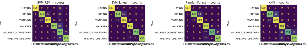
Figure 1 shows performance of four machine learning models: SVM RBF, SVM Linear, RandomForest, and KNN. For SVM RBF that did the worst, the recall for the walking, 0.83, is bad because it mistakes it for walking downstairs and the recall for walking upstairs is 0.89 because it also predicts walking downstairs. The precision for walking downstairs is the worst, at a 0.65. Walking, Upstairs, and Downstairs all have step-like patterns and similar magnitudes. RBF likely underperformed linear here because it overfitted local quirks. 

Random forest and KNN make pretty much the same errors, mistaking sitting for standing and mistaking walking and walking upstairs for walking downstairs. 

CNN performed better than RNN. The slightly better performance might be because CNN, which detects whether there are certain repetitive traits in motion, works better for classifying activities like walking than RNN that classifies based on how motion changes over the whole period. The LSTM emphasizes longer temporal dependencies and ordering; with a short window and the chosen hyperparameters, it likely needs more capacity or more epochs to close the gap. Indeed, our grid limited max epochs (the best RNN used the cap), suggesting the RNN may not have fully converged under our search budget, whereas the CNN’s optimization is easier and more parallel.

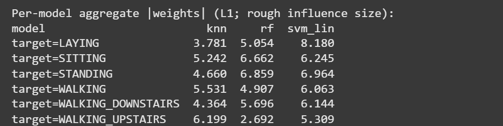
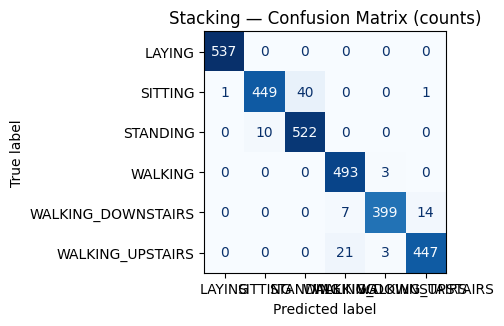
Stacking outperformed SVM linear. From the weights given to different models for different classes, it can be inferred that KNN is better than SVM linear in walking upstairs, random forest is slightly better than SVM linear for sitting, so stacking slightly improves upon linear SVM’s performance because it takes advantage of other models to predict classes where they outperform SVM linear. The confusion matrices in figure 3 back this up, showing how the biggest improvement from linear SVM to stacking is the recall for sitting, which is 0.88 for linear SVM and 0.92 for stacking. A downside is that it is more memory consuming compared to the classic models because it needs to manage 3 models and logistic regression. Given the accuracy gains, this cost is justified for applications that prioritize predictive quality; where memory or latency is tight, the linear SVM remains an exceptionally strong and compact baseline.

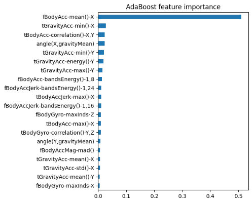
As shown in figure 4, adaboost with decision trees did comparatively well, outperforming random forest. The most important features were Gravity acceleration mean on X/Y/Z, which tells you the phone’s orientation relative to gravity. It’s useful for separating postures and body acceleration along axes, which helps separate movements. This is evidence that boosted trees capture strong, one-feature cues well.

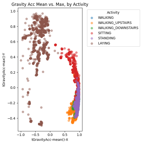
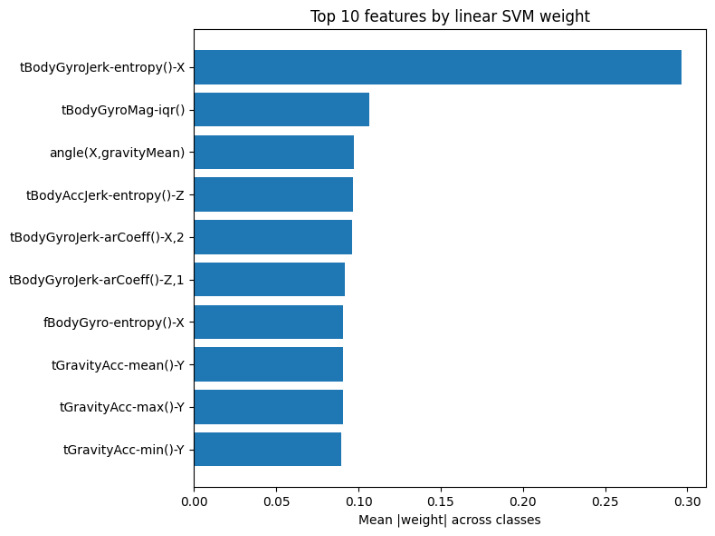
SVM linear performed the best out of the classical models. The classes are already almost linearly separable with the features. The scatterplot in figure 5 shows clear clusters—where A linear boundary (a weighted sum of a few of these stats) is enough to predict if a datapoint is laying or not. The horizontal axis shows the gravity acceleration along the phone’s X-axis. In the graph, when acceleration is negative, all datapoints are lying down. This makes sense because the phone is attached to the participants’ waist, so the x axis would be vertical and gravity would pull “downwards”. The vertical axis shows the maximum gravity acceleration along the phone’s Y-axis. Lying is higher than the rest and this might happen when they are lying down on their side. Figure 6 shows the top 10 features ranked by their mean weight across classes in a linear SVM (Support Vector Machine) model.The learned weights also align with sensor physics: gravity-related statistics separate static postures (LAYING/SITTING/STANDING), while gyro-based measures, how fast and in which direction the device is rotating for each axis, help with dynamic classes (WALKING and stairs). A repeated mistake on the confusion matrix is SVM predicting standing for sitting, which all the other classical models struggle with as well.

4. Conclusion

In this study, the simplest and most reliable takeaway is that linear SVM gave the best single-model results, and stacking several strong models together gave the best results overall. The CNN slightly beat the RNN because it is good at finding short, repeated motion patterns in the 128-step windows, while the RNN focuses more on long-range order that was less important here. The RBF SVM did not beat the linear SVM, likely because these engineered features are already close to linearly separable after scaling, so extra nonlinearity did not help. Random Forest and KNN were competitive but made similar mistakes on look-alike classes (sitting vs. standing, walking up vs. down). In terms of size, KNN uses the least memory, while stacking uses the most among classical models because it keeps three models plus a small combiner. Overall, our results suggest that simple margins (linear SVM) generalize well, and that combining models (stacking) can add small gains. For future work, the plan is to look into reducing “walking downstairs” false positives, and try out image recognition datasets in the human activity recognition domain.

References

[1]. Hammerla et al. (2016) Deep, Convolutional, and Recurrent Models for Human Activity Recognition using Wearables.
[2]. MDPI Paper (2020) Comparing Human Activity Recognition Models Based on Sensor Data.
[3]. Gaikwad et al. (2024) Benchmarking Classical, Deep, and Generative Models for Human Activity Recognition.
[4]. Ahmad et al. (2020) Human Activity Recognition using Multi‑Head CNN followed by LSTM.
[5]. Mathew et al. (2023) Human activity recognition using Single Frame CNN and ConvLSTM.
[6]. Khan & Hossni (2025) Comparative Analysis of LSTM Models Aided with Attention and Squeeze‑and‑Excitation Blocks for Activity Recognition (Scientific Reports)
Cite this article
Yang,Y.;Wang,X. (2025). In-depth Analysis of the Performance and Applications of Classical and Deep Learning Models under the UCI HAR Dataset. Applied and Computational Engineering,203,53-64.
Data availability
The datasets used and/or analyzed during the current study will be available from the authors upon reasonable request.
Disclaimer/Publisher's Note
The statements, opinions and data contained in all publications are solely those of the individual author(s) and contributor(s) and not of EWA Publishing and/or the editor(s). EWA Publishing and/or the editor(s) disclaim responsibility for any injury to people or property resulting from any ideas, methods, instructions or products referred to in the content.
About volume
Volume title: Proceedings of CONF-SPML 2026 Symposium: The 2nd Neural Computing and Applications Workshop 2025
© 2024 by the author(s). Licensee EWA Publishing, Oxford, UK. This article is an open access article distributed under the terms and
conditions of the Creative Commons Attribution (CC BY) license. Authors who
publish this series agree to the following terms:
1. Authors retain copyright and grant the series right of first publication with the work simultaneously licensed under a Creative Commons
Attribution License that allows others to share the work with an acknowledgment of the work's authorship and initial publication in this
series.
2. Authors are able to enter into separate, additional contractual arrangements for the non-exclusive distribution of the series's published
version of the work (e.g., post it to an institutional repository or publish it in a book), with an acknowledgment of its initial
publication in this series.
3. Authors are permitted and encouraged to post their work online (e.g., in institutional repositories or on their website) prior to and
during the submission process, as it can lead to productive exchanges, as well as earlier and greater citation of published work (See
Open access policy for details).