1. Introduction

Recommender systems have become indispensable to online platforms, supporting personalized services that enhance both user experience and commercial outcomes. Early collaborative filtering (CF) approaches, represented by matrix factorization, proved effective in practice but were limited in capturing nonlinear user–item relationships and were prone to exposure bias. Neural Collaborative Filtering (NCF) subsequently extended this paradigm by employing deep neural networks to model complex interactions, which markedly improved recommendation accuracy [1]. Building on this foundation, models such as Neural Tensor Factorization (NTF) and the Deep Interest Network (DIN) incorporated temporal dynamics and user interest heterogeneity, further enriching the modeling of user behavior [2,3].

Nevertheless, the problem of exposure bias in implicit feedback remains unresolved. Popular items tend to dominate recommendation lists, while equally relevant but less-exposed items are systematically overlooked, reducing both fairness and diversity. Although approaches such as inverse propensity scoring (IPS) and bandit-based exploration have been developed to alleviate this imbalance, finding an effective compromise among accuracy, fairness, and stability continues to present difficulties.

In light of these challenges, this study develops a stacked debiased NCF framework. The design combines IPS-weighted NCF with CatBoost under a stacking scheme, bringing together the representational advantages of neural networks and the robustness of tree-based learners. Empirical analysis shows that this hybrid approach improves predictive accuracy while reducing exposure bias, thereby offering fairer and more reliable recommendations for large-scale application scenarios [4].

2. Method

In recommendation systems, user click behavior tends to be highly sparse and unevenly distributed, especially at the hourly level or at specific product granularity. On the one hand, traditional deep learning methods (such as NCF) can capture complex user-product interactions, but when the sample is sparse or the data is unevenly distributed, it is difficult for the model to accurately estimate the preferences of certain users or products. On the other hand, click behavior is affected by conditions such as time, category, and user characteristics, and its probability distribution fluctuates greatly with time, which may lead to unstable predictions or overfitting of the model if left untreated.

In order to solve these problems, a variety of statistical and weighted features are introduced into the model input. Specifically: (1) by constructing multi-granularity CTR (Click-Through Rate) features to supplement the prior information of the model; (2) IPS (Inverse Propensity Scoring) and its improved form SNIPS were used to weight the samples to mitigate the exposure bias in the data; (3) Design a hybrid structure that combines depth model and tree model to give full play to the complementary advantages of the two in modeling complex interactions and processing category features.

Next, we will introduce the construction of CTR features, propensity estimation and weighting methods, and model design and training details.

2.1. Click-Through Rate (CTR)

Click-Through Rate (CTR) is an important prior signal in recommendation systems, but its empirical distribution often has significant time fluctuations, as shown in Figure 1. If the original CTR value is directly relied upon, it is easy to cause instability or even distortion in the prediction in sparse scenarios. To this end, the conditional CTR feature is constructed on the training set as an auxiliary input for the model to enhance robustness and alleviate data sparsity.

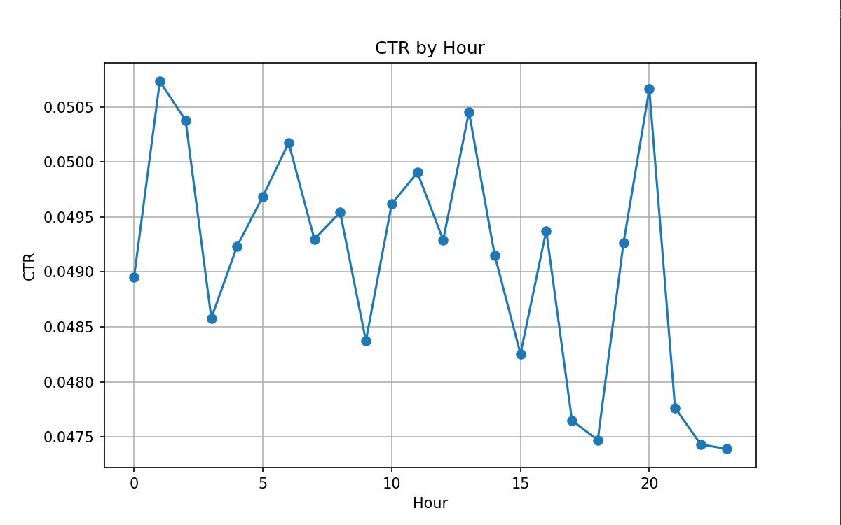
Specifically, for a condition grouping (such as user-hour, category-hour, or product-hour), a smoothed CTR is defined as:

$$ {CTR}_g=\frac{{clicks}_g+\alpha }{{imps}_g+\beta }$$(1)

Among them, clicks represents the number of user clicks, and imps represents the number of ad impressions. α and β are smoothing coefficients, which are used to balance the deviation and variance. In the implementation, we choose α=1 and β=3 to provide stable estimation in sparse scenarios while avoiding overfitting of low-frequency groupings.

In this study, three types of CTR features are constructed:

•User-hour CTR: Describes the user's active preferences at different time periods.

•Category-hour CTR: reflects the time dynamics at the category level;

•Item-Hour CTR: Captures short-term click trends for individual products.

When missing groupings appear in the test set, we use global CTR for padding to ensure consistency and prevent information leakage. By introducing these statistical features, the model can obtain more reasonable prior information in sparse or highly volatile data environments, thereby improving the stability and generalization ability of overall prediction.

It is important to note that relying solely on CTR features still does not completely eliminate the exposure bias inherent in recommendation logs. Therefore, in the subsequent method, we further introduce a correction mechanism based on propensity estimation and IPS/SNIPS weighting to improve the unbiased and robust prediction results while ensuring the efficiency of information utilization.

2.2. Exposure/propensity estimation and sample weighting (IPS/SNIPS/shear)

However, traditional recommendation log data has a strong exposure bias. To counteract this bias, we used propensity estimation based on historical frequency and used for sample weighting.

2.2.1. Propensity estimation (propensity)

We estimate the conditional exposure probability at coarse-grained context (hour, cate_id, pid) statistical frequencies in the training set:

$$ \widehat{p}\left(pid \right|hour, cate)=\frac{count(pid, hour, cate)}{count(hour, cate)}$$(2)

If the conditional probability is missing or very low, the occurrence rate of PID in the global training set will be used as a regression estimate of the global propensity p(pid). Final predisposition is defined as:

$$ {\widehat{p}}_i=\max \left(\widehat{p}\left({pid}_i \right|{hour}_i, {cate}_i\right),{\widehat{p}}_{global}\left({pid}_i\right),ϵ)$$(3)

2.2.2. IPS weighting, clipping, and normalization

Propensity-based IPS weights:

$$ w_i^{IPS}=\frac{1}{{\widehat{p}}_i}$$(4)

To control the variance explosion caused by extreme weights, crop the upper and lower bounds of the weights (e.g., clip to [0.2, 5.0]) and normalize the weights of all training samples to ensure that the weight table does not change the overall loss level:

$$ {\tilde{w}}_i=\frac{clip(w_i^{IPS},w_{min},w_{max} )}{\frac{1}{N}\sum _{j=1}^{N}clip(w_i^{IPS},w_{min},w_{max} )}$$(5)

2.2.3. SNIPS (Self-Normalizing IPS)

In NCF training, we use SNIPS-style weighted loss to further reduce variance:

$$ L_{SNIPS}\left(\theta \right)=\frac{1}{{\sum }_i{\tilde{w}}_i}\sum _i{\tilde{w}}_i·l(f_{\theta }\left(x_i\right),y_i)$$(6)

Where l is based on binary cross-entropy on a sample-by-sample basis. When SNIPS weights are used directly for PyTorch's dataset, the weighted loss is calculated in w during training (or directly replacing the sample with equivalent sampling weights).

2.3. Model design and training details

This subsection is divided into three subsections detailing the structure, loss design, optimization, and probabilistic calibration details of NCF, CatBoost, and Stacking.

2.3.1. Neural Collaborative Filtering (NCF)

Neural Collaborative Filtering (NCF) is a class of recommendation models that integrate deep learning methods with traditional collaborative filtering techniques [1]. The core idea is to replace the inner product operation in matrix factorization (MF) with neural networks, thereby capturing more complex and non-linear user–item interactions [1]. The NCF framework adopted in this study consists of four main components: the input and embedding layer, the interaction modeling layer, the fusion layer, and the output layer.

2.3.1.1. Input and embedding layer

The model input consists of unique identifiers (IDs) for users and items. Since the user–item interaction data is highly sparse, directly using IDs as features is inappropriate. Instead, user IDs and item IDs are first mapped into low-dimensional dense vectors through embedding:

$$ u=Embedding\left({ID}_u\right), v=Embedding\left({ID}_u\right)$$(7)

Where and represent the user and item embedding vectors, and  $$ u\in R^{d}v\in R^d$$ denotes the embedding dimension.

2.3.1.2. Interaction modeling layer

To capture both linear and non-linear interactions, NCF introduces Generalized Matrix Factorization (GMF) and Multi-Layer Perceptron (MLP) structures:

GMF Component: Preserves the intuition of traditional MF by modeling linear interactions through element-wise multiplication of user and item embeddings:

$$ z_{GMF}=u\odot v$$(8)

MLP Component: Concatenates the user and item embeddings and feeds them into a multi-layer neural network to capture non-linear relationships:

$$ z_{MLP}=({\varphi }_L···{\varphi }_2({\varphi }_1\left(\left[u\left|v\right]\right)\right))$$(9)

where [u∣∣v] denotes the concatenation operation and  $$ {\varphi }_i$$  is the non-linear activation function at the i-th layer.

2.3.1.3. Fusion layer

The outputs of GMF and MLP are then combined to leverage their complementary strengths. Specifically, the vectors are concatenated and projected into a joint latent space:

$$ \mathrm{z}=\left[z_{GMF}\right|\left|z_{MLP}\right]$$(10)

2.3.1.4. Output layer

The fused vector z is passed through a fully connected layer with a Sigmoid activation function to generate the predicted probability of user–item interaction:

$$ {\widehat{y}}_{uv}=\sigma \left(h^{T}z\right)$$(11)

where enotes the predicted preference score between user u and item v, and σ( $$ {\widehat{y}}_{uv}$$ ⋅) is the Sigmoid function.

2.3.1.5. Model training

The NCF model is trained by optimizing a cross-entropy loss function:

$$ L=-\sum _{(u,v)\in D}[y_{uv}log\left({\widehat{y}}_{uv}\right)+\left(1-y_{uv}\right)\log \left(1-{\widehat{y}}_{uv}\right)]$$(12)

where yuv is the ground truth label for user–item interaction (1 for interaction, 0 otherwise). Model parameters are updated via backpropagation using optimization algorithms such as Adam.

2.3.2. CatBoost (IPS-based tree model)

The main advantage of CatBoost as a Class II baseline model is the built-in processing of category features and robustness to high cardinality of categories. We also use IPS weights (normalized) as sample_weight in our CatBoost training.

Training process: Build a pool (train_X, labels, weights, cat_features=cat_idx) and use cb.fit(train_pool, eval_set=test_pool). Platt scaling (LogisticRegression) is performed after outputting the probability or using the penultimate day as a more stringent calibration set.

2.3.3. Stacking (meta = CatBoost)

To explore whether model fusion improves performance, we use a simple and commonly used two-layer stacking architecture:

Level 1: Trained with CatBoost's NCF and output the calibrated predicted probability y^NCF, y^CB. Calibration uses Platt scaling: Train a simple logistic regressor on the validation set on the first-level output, mapping the raw probability to the calibrated probability.

Level 2 (Meta): Use CatBoost as the meta-learner, input as two columns of features [y^NCF, y^CB], and the training target is the real label. If you want to continue considering the IPS weights of the Meta layer, CatBoost Meta can also receive sample weights.

The design leverages CatBoost's ability to capture nonlinear relationships and correct first-order bias to fuse complementary information from two basic learners.

In summary, the effectiveness of debias recommendation is systematically discussed through IPS-NCF, CatBoost model based on gradient lifting tree, and combined stacking fusion method. These methods not only mitigate exposure bias in traditional CTR predictions but also offer complementary advantages in modeling complex nonlinear intersum capture category featuresThe datasets, preprocessing steps, training/test division methods, and parameter settings used in the specific experiments are described in detail in Chapter 3 Experimental Design.

3. Experiment

This paper is experimentally verified on the "Taobao Display Click-through Rate Estimation" (Ali_Display_Ad_Click) dataset released by AlibabaThis section will explain from four aspects: dataset and feature construction, time segmentation and training/test division, experiment setup, and evaluation metrics.

3.1. Dataset and feature construction

The data used in this experiment is a Ali_Display_Ad_Click public dataset, covering the ad impression and click logs of approximately 1.14 million users over an 8-day period, totaling approximately 26 million records. Each sample contains the user ID, ad unit ID, timestamp, placement, and click tag (clk ∈ {0,1}). The data also comes with three types of feature tables: ad characteristics (ad_feature), user personas (user_profile), and user behavior logs (behavior_log). Among them, the advertising characteristics include category, delivery plan, brand and price; User portraits provide attributes such as gender, age level, consumption level, shopping depth, and occupation. The user behavior log records the user's browsing, add-on, favorite and purchase behavior within 22 days.

In order to ensure the quality of modeling, we first carried out strict missing value treatment on the original data. Specifically:

1)Delete missing records in key columns (user, adgroup_id, clk) directly;

2)If the relevant fields (brand, cms_segid, cms_group_id, final_gender_code, age_level, pvalue_level, shopping_level, occupation, new_user_class_level) are missing, they will also be deleted.

3)For user behavior features (beh_pv, beh_cart, beh_fav, beh_buy, beh_total), if there are null values, fill them with 0.

The code implementation uses chunk processing (chunksize=5,000,000) to clean it block by block to avoid memory overflow. For example:

chunk.dropna(subset=key_columns, inplace=True)

chunk.dropna(subset=user_profile_cols, inplace=True)

chunk[behavior_cols] = chunk[behavior_cols].fillna(0)

After processing, the original 26 million samples were reduced to approximately 7,003,565, and this data was used as the final modeling sample.

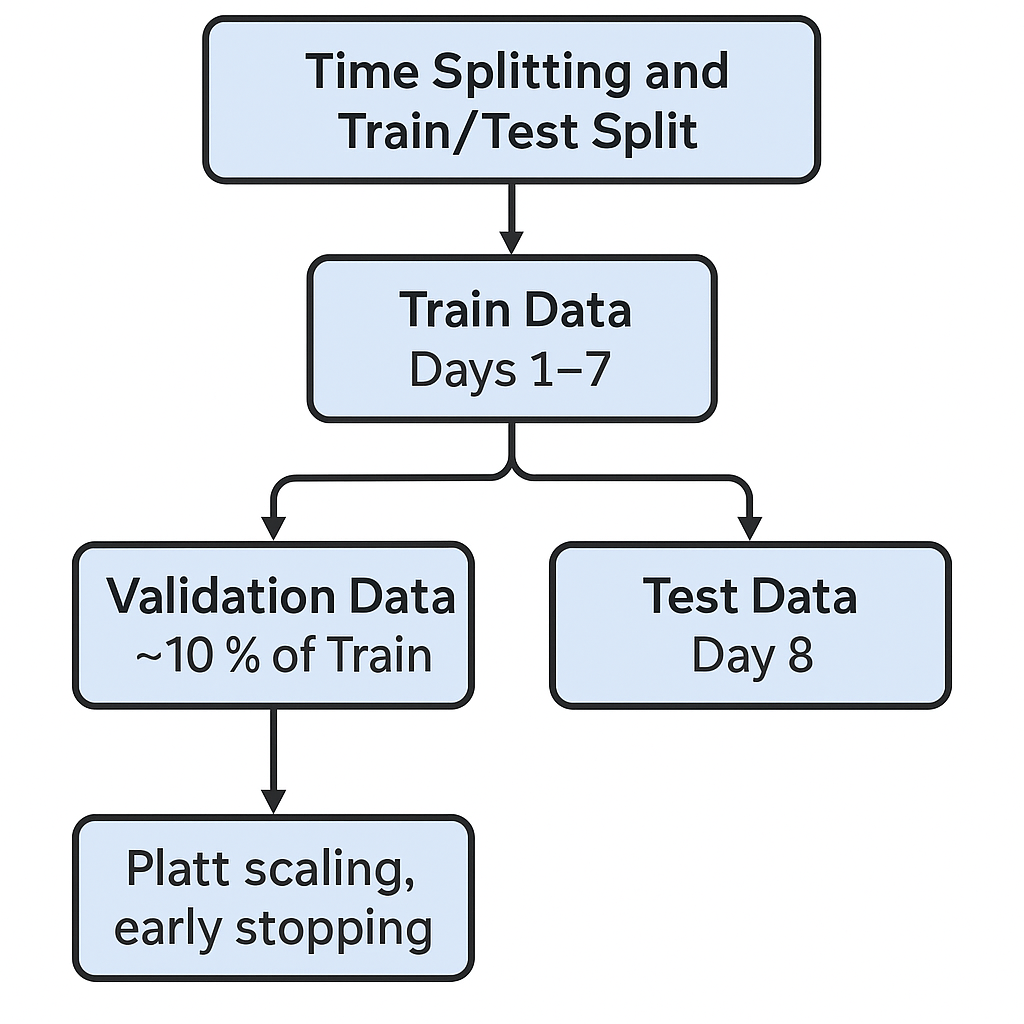
3.1.1. Temporal feature construction and data division

We convert timestamps to date and hour fields and further construct periodic time features (such as hour_sin, hour_cos, weekday_sin, weekday_cos) to capture the periodic patterns of user behavior. In terms of dataset division, the chronological order is followed: the first 7 days are used as the training set, and the 8th day is used as the test set to match the causal logic of the actual recommended scenarios.

3.1.2. Category feature coding and cross-features

In the feature engineering process, the LabelEncoder encoding of high-cardinality category features such as users, advertisements, categories, and delivery plans is first performed for subsequent model processing.

In the construction process of category crossover features, we combine statistical indicators to screen candidate features, rather than relying solely on human experience. Specifically, we calculated the following two metrics:

CTR_diff: Used to measure the ability of a feature to distinguish click behavior. It is defined as the difference between the maximum and minimum values of the click-through rate under different values of the feature, that is

$$ {CTR}_{diff}=\max \left({CTR}_g\right)-\mathrm{m}\mathrm{i}\mathrm{n}\left({CTR}_g\right)$$(13)

It can be seen that the larger the CTR_diff, the stronger the ability of the feature to distinguish the click behavior under different values.

high_freq_count: Used to measure the coverage of the feature in the training set, that is, the sum of the number of groups with the number of occurrences above a certain threshold for each value group. This metric is used to control sparsity, ensuring that the model does not produce erratic predictions due to rare values.

By calculating CTR_diff and high_freq_count, we can take into account both feature discrimination ability and sample distribution stability, which is an important basis for screening cross-features.

After sorting a total of 238 feature combinations in the dataset according to the above two numerical sizes (if the CTR_diff difference between the two features is ≤ 0.01, they are considered to be CTR_diff similar, and then the high_freq_count are compared to determine the priority; If the CTR_diff difference > 0.01, the CTR_diff larger trait is preferred), and some user attributes × brand/category combination traits (e.g., brand_shopping_level_bin, brand_new_user_class_level_bin) are in the top 30, showing high CTR differentiation ability. Other candidate crossover features (e.g., brand_age_level_bin, brand_occupation_bin, cate_id_final_gender_code_bin, cate_id_hour_cos_bin, cate_id_weekday_sin_bin) are not in the Top 30, but they still have some CTR differentiation within the Rank 30–60 range , and is stably distributed in the sample, which can provide complementary information for the model.

These characteristics also make sense logically for business:

•User attributes × Brand/category: Reflects the differences in product preferences of different user groups;

•Time characteristics × categories: Reflects click behavior patterns in different categories over different time periods.

Table 1 lists the final selected crossover features and their ranking in the CTR_diff ranking, so that readers can intuitively understand the basis and decision logic of our feature selection.

3.1.3. Statistical characteristics of CTR

Finally, we designed the CTR statistical features. The three dimensions of user-hour, category-hour, and placement-hour are aggregated on the training set, the smoothed click-through rate is calculated, and the results are mapped to the test set. For example, the user-hour CTR is constructed as follows:

g = train_df.groupby(['user','hour'])['clk'].agg(['sum','count']).reset_index()

g['user_hour_ctr'] = (g['sum'] + 1.0) / (g['count'] + 3.0)

train_df = train_df.merge(g[['user','hour','user_hour_ctr']], on=['user','hour'], how='left')

This method provides additional statistical prior information to the model while alleviating the sparseness problem.

3.2. Time partitioning and training/test division

In order to ensure the causal consistency and controllability of the experimental results, we adopt a strict time series partitioning strategy: the first 7 days of the dataset are selected as the training set, and the 8th day is used as the test set. This division method avoids future information leakage and is closer to the online application scenarios of actual recommendation systems.

3.3. Experimental setup

During the model training process, we uniformly set random seeds (42) to ensure reproducibility, and the optimizer uses AdamW and performs early stop monitoring on the training set to reduce the risk of overfitting. The following describes the implementation and parameter configuration of the three types of models.

3.3.1. IPS-NCF model

This model is based on the PyTorch implementation. First, we map users, advertisements, and cross-features into dense vectors through embedding layers, and then stitch them with continuous features such as time and behavior statistics and input them into multilayer perceptrons (MLPs). Introducing Inverse Propency Score (IPS) weighted binary cross-entropy loss during model training, combined with SNIPS and double robust estimation (DR), to mitigate data bias. The key parameters are configured as follows:

These settings are relatively stable in the early parameter adjustment. 64-dimensional embeddings strike a balance between computational overhead and expressive power, and four-layer MLP effectively captures higher-order nonlinear features. Dropout and weight decay further reduce the risk of overfitting, while the IPS combined with SNIPS+DR strategy ensures that the model has stronger generalization in data environments with selection bias.

3.3.2. CatBoost model

CatBoost directly leverages its native support for class features, avoiding the manual coding process and demonstrating good stability and efficiency in CTR prediction tasks. The key parameters are configured as follows:

The selection of parameters also comes from the pre-experimental results. The deep tree structure (depth=8) ensures sufficient expression ability, while the moderate learning rate and early stop strategy effectively prevent overfitting. 3000 iterations guarantee that the model achieves convergence while avoiding overtraining.

3.3.3. Stack the fusion model

In the fusion phase, we adopt a stacking strategy. The primary learner consists of IPS-NCF and CatBoost, and the output of the two is calibrated by probabilistic calibration (Platt scaling) and used as input features to train lightweight secondary models. The key parameters are configured as follows:

CatBoost was chosen as the secondary model due to its robustness and fast convergence speed for small-scale high-dimensional inputs. The lightweight configuration allows it to efficiently integrate prediction information from the first-level learner, thereby further improving the overall prediction accuracy and stability.

3.4. Evaluation indicators

To comprehensively measure recommendation performance, the following metrics are employed:

AUC (Area Under ROC Curve): Measures the model's ability to distinguish between clicked and non-clicked samples and is the primary evaluation metric.

$$ AUC=\frac{1}{N_{+}{N}_{-}}\sum _{i:y_i=1}\sum _{i:y_i=0}1(f\left(x_i\right)>f(x_j\left)\right)$$(14)

LogLoss: Measures the gap between the predicted probability and the true label;

$$ LogLoss=-\frac{1}{N}\sum _{i=1}^N[y_{i}log{\widehat{p}}_i+(1-y_i)\mathrm{l}\mathrm{o}\mathrm{g}(1-{\widehat{p}}_i)]$$(15)

Gini Coefficient (Gini): Measures the model's ranking consistency and is a complementary metric to AUC. It is related to AUC by the formula Gini=2×AUC−1, reflecting how well the model separates positive and negative samples.

$$ Gini=2·\frac{1}{N_{+}{N}_{-}}\sum _{i:y_i=1}\sum _{i:y_i=0}1\left(f\right(x_i)>f(x_j\left)\right)-1$$(16)

Where N+​ and N−​ are the numbers of positive (clicked) and negative (non-clicked) samples, respectively, and f(x) is the predicted score for sample xxx.

Lift @ K% (Lift@K%): Measures the improvement of the model in identifying positive samples within the top K% of predicted scores compared to random selection. It reflects the business impact of the recommendation system, e.g., how many more clicks can be captured by showing the top K% recommended items.

$$ Lift@K\%=\frac{CTR of top K\% ranked samples}{CTR of all samples}=\frac{\frac{1}{\left|S_K\right|}{\sum }_{i\in S_K}{y}_i}{\frac{1}{N}{\sum }_{i=1}^N{y}_i}$$(17)

Where $$ S_K$$ ​ is the set of samples in the top K% by predicted score,  $$ y_i $$ is the true label (1 for click, 0 for no click), and N is the total number of samples.

In summary, this study takes into account both robustness and rationality in data processing and experimental settings. The independence of training and testing is ensured through time segmentation, and feature engineering includes both basic behavioral and temporal features, as well as cross-feature and CTR statistics to improve expressiveness. At the model level, we set up three types of methods: IPS-NCF, CatBoost and stacked fusion, and took into account the theoretical basis and pre-experimental performance in the parameter selection. This design not only lays a solid foundation for subsequent experimental analysis, but also ensures the fairness and credibility of the comparison results.

4. Results and analysis

To further understand the source of the performance of each model, we first analyzed the loss and sequencing power trends of NCF and IPS-NCF during training (Figure 3). Overall, the training and test losses of NCF gradually decreased with training iteration, and the model convergence was stable and there was no obvious overfitting. After the introduction of IPS weighting, IPS-NCF converged faster in the initial training stage and ultimately had lower test losses, indicating that the weighted sample strategy improved the sensitivity of the model to low-exposure samples and made the prediction more robber.

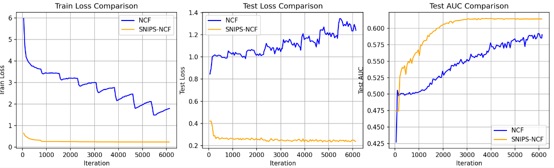
In terms of the sorting ability of the test set, the AUC of NCF gradually increases with training, while the AUC of IPS-NCF is always higher than that of NCF, indicating that IPS weight improves exposure bias and enhances the ranking ability of the model. Although the test loss may fluctuate slightly in the intermediate training phase, the final convergence trend is good, and the AUC is stable at a high level, indicating that the weighting strategy does not affect the overall training stability while improving the discriminatory ability of low-exposure samples.

The final performance of the four types of models is further compared on the test set:

From the results, the AUC of CatBoost (0.63403) is significantly higher than that of the NCF alone (0.59275), while Stacking further reaches 0.64872, indicating that the fusion model has a significant advantage in sorting ability (the higher the AUC, the better the model can distinguish between positive and negative samples, and the better the sorting effect). The introduction of IPS-weighted NCF (IPS-NCF) increased the AUC to 0.61398, indicating that weighting can partially improve the under-sorting caused by sample exposure bias.

In terms of probability quality index (LogLoss), the original LogLoss of NCF is 0.21340, reflecting that there is a certain deviation in probability estimation. After IPS-NCF, LogLoss was reduced to 0.20138, showing that the weighting improved the model's sensitivity to low-exposure samples and improved the average probability error to a certain extent, but still inferior to CatBoost (0.18865). Stacking finally achieved the lowest LogLoss (0.18692), indicating that its probabilistic prediction stability and reliability were the best (LogLoss). smaller means that the predicted probability is closer to the true probability distribution). This conclusion is echoed in the Gini coefficient: Stacking's Gini is 0.29744, which is higher than CatBoost's 0.26806 and IPS-NCF's 0.22797 (Gini = 2*AUC-1, which is essentially a supplementary quantitative measure of rank consistency).

From a business perspective, the Top-K indicators (Lift@10%, Lift@20%) show the same trend: CatBoost Lift@10% is 1.98198, Stacking is up to 2.13098, and Lift@20% is up from 1.73952 to 1.81756. This means that in scenarios with limited referral slots or limited resources (such as a few referral slots in front of the homepage or a promotional push list), the Stacking model can reach more real clicks or converting users with the same push volume than a single CatBoost, which has direct business value (top-10% coverage efficiency improvement of about 7%).

Combining the probability distribution in Figure 4 and Figure 5 can be further combined to explain these numerical differences more intuitively. Figure 4 (NCF) shows that the distribution of the NCF raw output (blue dotted line) is more scattered, with a relatively high probability long tail in the right tail (i.e., the model over-confidence on some samples), which amplifies LogLoss (because the high probability prediction penalty is heavier for a small number of errors); After Platt/Logistic calibration (solid orange line), the distribution is significantly contracted to the left and more concentrated, indicating that the calibration reduces the high probability of overconfidence and brings the predicted probability closer to the true frequency, resulting in improved LogLoss, but limited effect on the relative order (ordering), so the AUC does not change much.

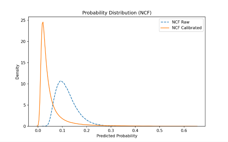
Figure 4.2 (CatBoost) shows that the original probability distribution of the tree model is relatively concentrated and smooth, and the difference before and after calibration is small, indicating that CatBoost has generated robust probability estimation through leaf-end frequency or regularization mechanism during training, so it naturally has an advantage in LogLoss.

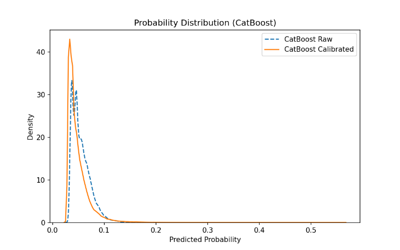
Comparing the two graphs, NCF is better at providing "strong relative scoring signals" (high variance but high information), while CatBoost provides "robust and low-variance probability estimation"; The improvement in stacking comes from the dynamic weighting of the output of the meta-learner: more trust in NCF's discriminant signals in some user/product/time windows (increased AUC), and more reliance on CatBoost's robust probability in other cases (reduced LogLoss), and the two complement each other to form a comprehensive advantage.

In general, this experiment reveals the following laws: firstly, the depth model is prone to the problem of excessive probability concentration when not calibrated, and the probability output can be effectively improved through calibration and IPS weight adjustment. Secondly, the tree model has natural advantages in classification and statistical feature modeling, and the improvement space for probability output is relatively limited. Finally, the stacked fusion strategy can give full play to the complementarity of different models and achieve comprehensive optimal results in terms of sorting performance and reliability of probability output.

5. Conclusion

This study focuses on the exposure bias problem in click-through rate prediction and proposes a stacked, debiased NCF model. The research addresses three aspects: first, by constructing spatiotemporal statistical features and cross features, it effectively mitigates the challenges posed by data sparsity and dynamic variations; second, by incorporating inverse propensity weighting (IPS/SNIPS), it significantly reduces the bias caused by uneven historical exposure distributions during training; finally, by combining CatBoost with NCF in a stacking framework, the model captures high-order nonlinear interactions while maintaining the robustness and interpretability of tree-based models. Experimental results show that using NCF or CatBoost alone improves predictive performance but has inherent limitations; IPS weighting enhances both prediction accuracy for low-exposure samples and ranking performance (AUC); the stacked model achieves the best results in AUC, LogLoss, and business-related Top-K coverage metrics, covering more real clicks and conversions in limited recommendation slots or resource-constrained scenarios, demonstrating clear practical value. These findings indicate that the deep interaction features captured by NCF complement the robust probability estimates of CatBoost, and the stacking model dynamically integrates both strengths through a meta-learner, achieving overall improvements in ranking, probability reliability, and business efficiency, providing an effective solution for debiased recommendation tasks.

Based on these results, this study has direct practical significance. In e-commerce advertising and large-scale personalized recommendation systems, the stacked debiased model can improve click and conversion efficiency, enhance user experience, and strengthen platform competitiveness. It also offers an actionable approach to mitigating historical exposure bias, contributing to fairness and stability in recommendation systems, and providing theoretical and practical support for decision-making in high-traffic, complex scenarios. Building on this foundation, future work will further extend the model’s applicability and robustness. Specifically, incorporating multimodal inputs (e.g., text and images), exploring more robust debiasing strategies based on causal inference or adversarial training, enhancing interpretability and fairness, and developing online or incremental learning mechanisms for real-time recommendation scenarios can further improve predictive performance and recommendation fairness. These enhancements will provide more comprehensive and deployable solutions for complex, high-volume recommendation systems, further increasing the practical value of this research.

References

[1]. Li, P., Noah, S. A. M., & Sarim, H. M. (2022). Convolutional Transformer Neural Collaborative Filtering. National University of Malaysia.
[2]. Wu, X., Shi, B., Dong, Y., Huang, C., & Chawla, N. V. (2018). Neural Tensor Factorization. Proceedings of the 24th ACM SIGKDD International Conference on Knowledge Discovery & Data Mining (KDD’18). https: //doi.org/10.1145/nnnnnnn.nnnnnnn
[3]. Zhou, G., Song, C., Zhu, X., Fan, Y., Zhu, H., Ma, X., Yan, Y., Jin, J., Li, H., & Gai, K. (2018). Deep Interest Network for Click-Through Rate Prediction. Proceedings of the 24th ACM SIGKDD International Conference on Knowledge Discovery & Data Mining (KDD’18). https: //github.com/zhougr1993/DeepInterestNetwork
[4]. Li, P., Li, X., & Zhu, X. (2025). Neural Collaborative Filtering Recommendation Model for De-Exposure Bias Based on Fused Rewards. Application Research of Computers, 42(1), 78–85. https: //doi.org/10.19734/j.issn.1001-3695.2024.05.0184
Cite this article
Fang,Y.;Yang,H. (2025). Stacking Outperforms in Debiased Neural Collaborative Filtering: A Comparative Study of IPS-Weighted NCF and Tree-Based Models for Exposure-Biased CTR Prediction. Applied and Computational Engineering,210,70-84.
Data availability
The datasets used and/or analyzed during the current study will be available from the authors upon reasonable request.
Disclaimer/Publisher's Note
The statements, opinions and data contained in all publications are solely those of the individual author(s) and contributor(s) and not of EWA Publishing and/or the editor(s). EWA Publishing and/or the editor(s) disclaim responsibility for any injury to people or property resulting from any ideas, methods, instructions or products referred to in the content.
About volume
Volume title: Proceedings of CONF-MLA 2025 Symposium: Intelligent Systems and Automation: AI Models, IoT, and Robotic Algorithms
© 2024 by the author(s). Licensee EWA Publishing, Oxford, UK. This article is an open access article distributed under the terms and
conditions of the Creative Commons Attribution (CC BY) license. Authors who
publish this series agree to the following terms:
1. Authors retain copyright and grant the series right of first publication with the work simultaneously licensed under a Creative Commons
Attribution License that allows others to share the work with an acknowledgment of the work's authorship and initial publication in this
series.
2. Authors are able to enter into separate, additional contractual arrangements for the non-exclusive distribution of the series's published
version of the work (e.g., post it to an institutional repository or publish it in a book), with an acknowledgment of its initial
publication in this series.
3. Authors are permitted and encouraged to post their work online (e.g., in institutional repositories or on their website) prior to and
during the submission process, as it can lead to productive exchanges, as well as earlier and greater citation of published work (See
Open access policy for details).