1. Introduction

The great evolution of artificial intelligence in the past decade has been attributed to the popularity of emerging information technologies such as big data and cloud computing and the enhancement of hardware devices that allow it to run on graphics processors rather than CPUs, which run far more efficiently than before. At the same time, with the release of policies such as “U.S. Department of Defense Artificial Intelligence Strategy Summary 2018 - Using Artificial Intelligence for Security and Prosperity” and “China's Guidance of the State Council on Actively Promoting ‘Internet+’ Actions”, etc., are extremely powerful in attracting talent and outstanding companies to participate in AI research and development. Now, the cell phone's face recognition, intelligent recognition and other functions are the symbols of artificial intelligence’s lightweight applications and great success.

Computer vision is a popular area of artificial intelligence, and its development mainly has the following stages. In the 1950s, the discovery of the structure of the visual function column laid the foundation for computer vision. The image scanner transflows the real image into a numerical type, which makes the computer able to analyze images. In the 1960s, Lawrence Roberts, "machine perception of three-dimensional solids", after which two-dimensional images can also describe three-dimensional objects. In the 1970s, computer vision’s theoretical framework was initially established, and MIT opened related courses. In the 1980s, computer vision was first applied, and the prototype of the neural network was born [1]. In the 1990s, CS research focus shifted to image recognition. In the early 21st century, image feature engineering and high-quality datasets with labeling were born, and the concept of deep pervasive networks was proposed. From 2010 to the present, deep convolution has been in full bloom, and networks such as ResNet [2] and GAN [3] have been proposed one after another. These models have been successfully applied in many domains, e.g., the traffic domain [4, 5] and the financial domain [6]. Along with the rapid development of computer vision, some of the problems are gradually exposed. Deep neural networks effectively improve the prediction accuracy, while the extremely high requirements for data with effective labeling make its training costs rise. The real situation is variable, and there may be noise interference such as light, angle, and distortion [7, 8]. As the number of parameters increases, the computing time also increases, which means more computing power is needed.

Although computer vision faces the above problems, its development is still rapid and is widely used in image generation and classification. For example, OpenAI has achieved great success in generating images, and deep neural networks are used for the transcription of Spanish historical handwritten documents [9]. With the accelerating improvement of computer vision, the archaeological industry and related literary creators can apply it in the areas of artifact identification, restoration and antique style creation.

In this paper, we use an open ancient handwritten recognition dataset Oracle-MNIST [10], try a series of CNNs such as ResNet, VGG [11], ViT [12], AlexNet, EfficientNet and many other deep learning models, and experience such as voting, bagging [13], snapshot and other ensemble learning methods [14]. Considering the parameters, running time and the most important target—accuracy—it is found that the simple CNN model trained as a snapshot performs best, which is better than the ResNet model with a snapshot, and the accuracy of recognition reaches 97.007%, even if it is not as well as voting’s accuracy of approximately 97.110%, but it only costs 112.644 seconds, while the latter costs 1013.048 seconds.

The arrangement of this paper is as follows. Section 2 discusses the related work. Section 3 introduces the datasets. Section 4 describes the methods and models. Section 5 shows the setting and results of the experiments. In Section 6, we will conclude and come up with some ideas that may help enhance the accuracy.

2. Related works

In this article, we mainly use the CNN model, which has been proven effective for handwritten characters recognition [15-17]. Therefore, it is meaningful to briefly explain its development and basic principles before launching. In 1998, as a pioneer, LeNet was created; it has a seven-layer network structure and uses tanh as its activation function. After that, CNN was dormant for a decade because of its excessive demand for computing power until the emergence of AlexNet, which won the imageNet2012 championship in one fell swoop. On the basis of summarizing the experience of predecessors, it reused ReLu as the activation function and proposed the dropout layer to prevent overfitting. Subsequently, VGG deepened the number of layers on the basis of AlexNet and demonstrated the use of convolution kernels (mainly 3 * 3) to increase the depth of the network and the accuracy of the model. There is a positive correlation, which has also been widely used for feature extraction. ResNet in 2015 pioneered the residual module to solve the degradation problem in the process of increasing network depth. Later, DenseNet used dense connections to alleviate the problem of gradient disappearance while strengthening feature propagation, encouraging feature reuse, and greatly reducing the number of parameters. Vision Transformer, proposed by the Google team in 2020, is based on the self-attention mechanism. Inspired by Transformer in NLP, the image is divided into patches, and the linear embedding sequence of these image patches is used as the input of Transformer. As a new work of 22 years, Vision GNN has skillfully applied graph neural networks to image classification and achieved excellent results.

With the continuous improvement and expansion of CNNs, their accuracy has increased. For example, the accuracy of the heterogeneous ensemble with a simple CNN reached 99.91% on the classical dataset MNIST. At present, CNNs have been used for tomato disease detection [18] and classification, mechanical fault detection, and protection of vehicle network standard CAN, which proves the success of CNNs. The exploration of historical handwritten documents explored in this paper is also based on CNN and has achieved satisfactory accuracy. All of these factors make the CNN a mature model.

As an ancient civilization, there were oracle bone inscriptions in China as early as three thousand years ago [19]. The Chinese history and cultural heritage contained in oracle bone inscriptions have attracted many scholars to further study it, which has become a major research hotspot in the field of history and culture.

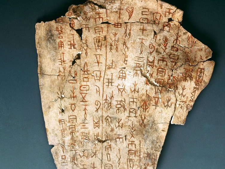
Figure 1. Oracle characters are the oldest hieroglyphs in China.

We encounter several major difficulties in the application of oracle bone inscription recognition, which has a negative impact on accuracy. 1 The physical conditions of oracle bone inscriptions, most of which are bones or stones, show different types of degradation after thousands of years, such as weathering, fading, stains, shadows and poor contrast in the writing part, and because it is scanned from the surface of real oracle bone inscriptions, it has unique noise. 2 The number of samples in each character may vary greatly from each other (data imbalance), forcing the robustness of the selected model to be high. 3 The words that may exist in ancient historical texts are not included in the current dictionary library. 4 The handwriting style of ancient Chinese characters is so changeable that even humans may make a mistake.

3. Description of the Dataset

The Oracle-MNIST dataset contains 30,222 oracle character images, 10 categories in total. All of these data come from the YinQiwenyuan website. These oracle bone inscriptions are scanned from the surface of the real oracle bone inscriptions, which are as difficult as the above ancient character recognition and have large noise. To facilitate the experiment, the image did not take enhancement measures. The raw data are shown in Table 2. As we can see, the same word has different types and writing styles.

4. Models and methods

In the experiments, we intend to focus on the following models: ResNet and two simple CNNs defined in the paper, which are named M3 and Com2 [20].

The residual block in ResNet adopts two layers of convolution layer and standard layer of 3 * 3 convolution kernel. If the step size is 1, the 1*1 convolution kernel is used for downsampling. Its network structure takes a 3*3 convolution kernel to convolute after two-dimensional batch processing and ReLU activation and window for (2,2) maximum pooling, using 8 residual blocks and putting the result into average pooling. The final layer is the full connection layer, and then the predicted label will be made.

M3 consists of ten convolutional layers and one fully connected layer. First, the input is taken as input x for (x-0.5) * 2. In each convolution layer, two-dimensional convolution and two-dimensional batch normalization are performed, and then ReLU activation is applied. In this experiment, it is found that the experimental effect is better when the convolution kernel is 3, so the convolution kernel is 3*3. The fully connected layer uses 1D batch processing for full connection and does not use dropout. In this experiment, M5 and M7 with similar structures but different convolution kernels are adopted. The essential difference between M5 and M7 is that the different sizes of the convolution kernel make the reduction of each convolution feature map different, so that the number of convolution layers is different.

Com2 is similar to the above model. But it uses a fixed 5 * 5 convolution kernel. After the two-dimensional convolution is performed and the window is filled with a window that has a size of 2, turn the result into the maximum pooling of the window, after which each feature mapping becomes the original 1/2. After 4 convolution layers, the matrix is changed from [0,1,2,3] to [0,2,3,1], that is, the number of image features is moved forward. The difference between Com1 and Com3 is the number of convolution layers.

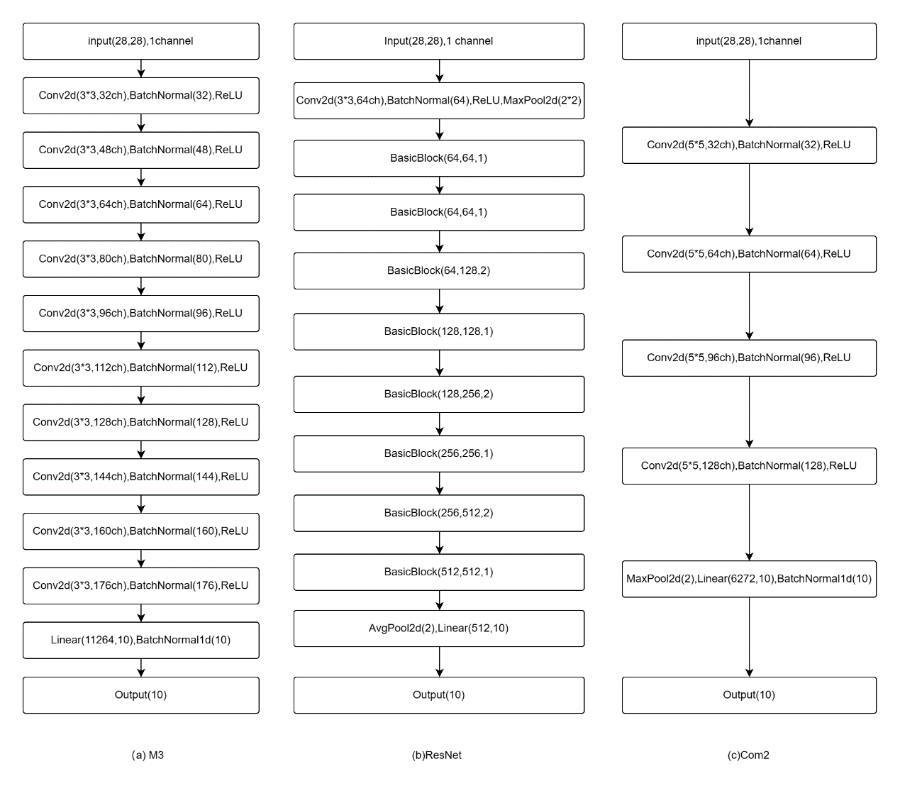
Figure 2. Network models used for Oracle-MNIST.

This experiment found that voting, bagging and snapshot can effectively improve the accuracy of the model. The following is a brief description of the three ensemble learning methods.

Voting can be divided into two categories: hard voting and soft voting. The hard voting uses the classification of each model and the class with the maximum value as the output, while the soft voting outputs the class output probability and the class with the maximum value through each model.

The full name of bagging is bootstrap aggregating. For a given training sample, the training sample is extracted from the training sample in each round by means of put-back sampling. The sample set is obtained by repeated sampling, and the sample sets are independent of each other. Voting is performed after model prediction based on each sample set.

Snapshot, using SGDR as its learning strategy. The SGDR strategy is divided into two parts. First, the learning rate is reduced from the maximum to the minimum according to cosine annealing (CosineAnnealing) and then reset to the maximum. The model converges to the local optimum when each cosine annealing is completed, so that the rest of the local optimum can be found after the reset, so that a weak model can be obtained after each training. A snapshot in the training process can greatly reduce the running time.

5. Discussion

In this experiment, the training set contains 27222 images, and the testing set contains 3000 images. The proportion of the total image divided into training and testing is approximately 9: 1. It is proposed to take accuracy as the main evaluation index and consider the number of model parameters and model running time at the same time. The programming language is Python, using some designed packages such as torch, torchensemble, numpy, and timm. The computer configuration is 11800 h + 3070 laptop, and all of the experiments are based on CUDA. The following experiments use the Adam optimizer.

Table 2. Training data and test data.

To compare fairly, the following results are computed on the same computer, every time having the same training data and test date, and the number of epochs is 15 if there is no mention. After one training, we will empty the CUDA memory.

Table 3. The results of some models without ensemble learning.

Table 4. The results of some models without ensemble learning.

Net1-3 is the CNN model provided by the author of the dataset. vit uses ‘vit _ tiny _ patch16 _ 224’ concluded in the timm package, and regnet uses ‘regnetv _ 040’ in the timm package. Pnasnet uses ‘spnasnet _ 100’ in the timm package, efficient uses ‘efficientnet _ b0’ in the timm package, tnt uses ‘tnt _ s _ patch16 _ 224’ in the timm package, and ghostnet uses ghostnet _ 050 in the timm package. The above networks did not use training parameters. Several phenomena are found here: 1. The p value of the parameter quantity and the model accuracy is 0.208, which is greater than 0.05, indicating that there is no significant relationship between the two. For example, the Com3 parameter has the best performance, and the number of its parameters is 835204, while the accuracy rate is 95.06%, the ResNet accuracy rate is 94.288%, which is slightly inferior to Com3, but the number of parameters reaches 111758182. There is a significant relationship between the number of parameters and the training time, and the p value is 0.001.3. For the Oracle-MNIST dataset, some newly promoted network performances are general, such as VIT and GhostNet. The performance of CNNs varies greatly for different datasets.

Tabel 5. Test for between-subjects effects.

Then, we use ensemble learning to improve the models’ accuracy, all of which have 10 base estimators and 15 epochs. First, we use voting. As shown in the following table, the training times are almost ten times, and the parameters are also up to ten times, while there are apparent improvements in each model. As we can see, the accuracy of Com2 achieved 97.144%, with an increase of 4.064%, and M3 and ResNet achieved 96.707%, better than Net1-3. To streamline the experiment, we will examine Com2, ResNet and M3 in the other ensemble learning.

Table 6. The results of some models with voting, epoch=15.

Table 7. The results of some models with voting, epoch=15.

Compared with fusion and bagging, we find that bagging is good at improving the accuracy, while fusion can increase the training time, each of which has its own benefits.

Due to its special training methods, Snapshot’s epoch must be a multiple of the base estimators, so we use 20 epochs instead of 15, as described above. Snapshot is a quite efficient ensemble learning method in this experiment. Com2 costs only 112.644 seconds and has a surprising accuracy of 97.007%, which means that high efficiency in training with minimal accuracy loss is possible.

Table 8. The results of some models with bagging or fusion,epoch=15.

Table 9. The results of some models with Gradient Boosting or snapshot.

6. Conclusion

In this paper, we use many CNNs and ensemble learning methods to improve the accuracy of Oracle-MNIST dataset classification. Considering the time, the model parameters and the most important target accuracy, the simple CNN named Com2 with a snapshot performed the best and achieved an accuracy of 97.007%, which was better than that of Net1-3, which was given by the dataset’s author. However, research on this dataset and Oracle-MNIST can still have a significant improvement by enlarging the training and test data, exploring more models or ensambling different models, e.g., graph-based models [21, 22].

References

[1]. Chen, S. S., & Zhang, M. (1988, March). Adaptive (neural network) control in computer-integrated-manufacturing. In Applications of Artificial Intelligence VI (Vol. 937, pp. 470-473). SPIE.
[2]. He, K., Zhang, X., Ren, S., & Sun, J. (2016). Deep residual learning for image recognition. In Proceedings of the IEEE conference on computer vision and pattern recognition (pp. 770-778).
[3]. Goodfellow, I. J., Pouget-Abadie, J., Mirza, M., Xu, B., Warde-Farley, D., Ozair, S., ... & Bengio, Y. (2014). Generative Adversarial Networks. arXiv preprint arXiv:1406.2661.
[4]. Jiang, W., & Zhang, L. (2018). Geospatial data to images: A deep-learning framework for traffic forecasting. Tsinghua Science and Technology, 24(1), 52-64.
[5]. Zheng, Y., & Jiang, W. (2022). Evaluation of Vision Transformers for Traffic Sign Classification. Wireless Communications and Mobile Computing, 2022.
[6]. Jiang, W. (2021). Applications of deep learning in stock market prediction: recent progress. Expert Systems with Applications, 184, 115537.
[7]. Zhou, H., Xiong, H., Li, C., Jiang, W., Lu, K., Chen, N., & Liu, Y. (2021). Single image dehazing based on weighted variational regularized model. IEICE TRANSACTIONS on Information and Systems, 104(7), 961-969.
[8]. Zhou, H., Zhang, Z., Liu, Y., Xuan, M., Jiang, W., & Xiong, H. (2021). Single Image Dehazing Algorithm Based on Modified Dark Channel Prior. IEICE TRANSACTIONS on Information and Systems, 104(10), 1758-1761.
[9]. Granell, E., Chammas, E., Likforman-Sulem, L., Martínez-Hinarejos, C. D., Mokbel, C., & Cîrstea, B. I. (2018). Transcription of spanish historical handwritten documents with deep neural networks. Journal of Imaging, 4(1), 15.
[10]. Wang, M., & Deng, W. (2022). Oracle-MNIST: a Realistic Image Dataset for Benchmarking Machine Learning Algorithms. arXiv preprint arXiv:2205.09442.
[11]. Simonyan, K., & Zisserman, A. (2014). Very deep convolutional networks for large-scale image recognition. arXiv preprint arXiv:1409.1556.
[12]. Dosovitskiy, A., Beyer, L., Kolesnikov, A., Weissenborn, D., Zhai, X., Unterthiner, T., ... & Houlsby, N. (2020). An image is worth 16x16 words: Transformers for image recognition at scale. arXiv preprint arXiv:2010.11929.
[13]. Breiman, L. (1996). Bagging predictors. Machine learning, 24, 123-140.
[14]. Zhou, Z. H. (2012). Ensemble methods: foundations and algorithms. CRC press.
[15]. Jiang, W. (2020). MNIST-MIX: a multi-language handwritten digit recognition dataset. IOP SciNotes, 1(2), 025002.
[16]. Jiang, W. (2020, May). Evaluation of deep learning models for Urdu handwritten characters recognition. In Journal of Physics: Conference Series (Vol. 1544, No. 1, p. 012016). IOP Publishing.
[17]. Jiang, W., & Zhang, L. (2020). Edge-siamnet and edge-triplenet: New deep learning models for handwritten numeral recognition. IEICE Transactions on Information and Systems, 103(3), 720-723.
[18]. Kibriya, H., Rafique, R., Ahmad, W., & Adnan, S. M. (2021, January). Tomato leaf disease detection using convolution neural network. In 2021 International Bhurban Conference on Applied Sciences and Technologies (IBCAST) (pp. 346-351). IEEE.
[19]. Flad, R. K. (2008). Divination and power: a multiregional view of the development of oracle bone divination in early China. Current Anthropology, 49(3), 403-437.
[20]. An, S., Lee, M., Park, S., Yang, H., & So, J. (2020). An ensemble of simple convolutional neural network models for MNIST digit recognition. arXiv preprint arXiv:2008.10400.
[21]. Jiang, W., & Luo, J. (2022). Graph neural network for traffic forecasting: A survey. Expert Systems with Applications, 117921.
[22]. Jiang, W. (2022). Graph-based deep learning for communication networks: A survey. Computer Communications, 185, 40-54.
Cite this article
Wang,Z. (2023). Ancient character recognition with deep learning techniques. Applied and Computational Engineering,9,194-203.
Data availability
The datasets used and/or analyzed during the current study will be available from the authors upon reasonable request.
Disclaimer/Publisher's Note
The statements, opinions and data contained in all publications are solely those of the individual author(s) and contributor(s) and not of EWA Publishing and/or the editor(s). EWA Publishing and/or the editor(s) disclaim responsibility for any injury to people or property resulting from any ideas, methods, instructions or products referred to in the content.
About volume
Volume title: Proceedings of the 2023 International Conference on Mechatronics and Smart Systems
© 2024 by the author(s). Licensee EWA Publishing, Oxford, UK. This article is an open access article distributed under the terms and
conditions of the Creative Commons Attribution (CC BY) license. Authors who
publish this series agree to the following terms:
1. Authors retain copyright and grant the series right of first publication with the work simultaneously licensed under a Creative Commons
Attribution License that allows others to share the work with an acknowledgment of the work's authorship and initial publication in this
series.
2. Authors are able to enter into separate, additional contractual arrangements for the non-exclusive distribution of the series's published
version of the work (e.g., post it to an institutional repository or publish it in a book), with an acknowledgment of its initial
publication in this series.
3. Authors are permitted and encouraged to post their work online (e.g., in institutional repositories or on their website) prior to and
during the submission process, as it can lead to productive exchanges, as well as earlier and greater citation of published work (See
Open access policy for details).