1. INTRODUCTION

Coronavirus disease 2019, known as COVID-19, is a newly emerged epidemic which was spread in many countries worldwide since December 2019. There was no vaccine when it appears, and it could be easily transmitted by breathing the droplet containing the virus. More importantly, it could cause the death by exerting the negative effect on lung and triggering diseases such as pneumonia; bronchitis; and ARDS (acute respiratory distress syndrome) [1]. In order to protect people from COVID-19 and prevent the transmission, there are many governments asking citizens to wear the mask and keep the certain social distance from each other. Some countries, such as China, choose to isolate those who are infected and even the whole community of which the infected people living in, while they also curb the movement within the country and frequently enforce people to do COVID test. These various inconveniences caused by COVID-19 have changed our life to large extent. On the other hand, social media is always a place for people to share their different opinions conveniently. Therefore, when there is a dataset including tens of thousands of Twitter posts labelled manually with sentiment labels and those posts are all about COVID-19, it is worthy to investigate it with sentiment analysis, which is a branch of Natural Language Processing (NLP) [2]. As mentioned before, there was no vaccine for COVID-19 because it was new, and same reason applies to deep learning – This topic is never trained by any pre-training models, which is good for testing if the learning ability of current models is really strong as it seems to be.

When it comes to NLP, Recurrent Neural Network (RNN) is the most reasonable choice to be the base of the model, because RNN, unlike other classes of artificial neural network, could process variable number of inputs, which is always the case for processing language. In this part, we have the methods from the simple one-hot encoding, which only works well with data that have no relationship, to more reasonable methods, such as Bag of Words, Bag of N grams, TD-IDF, and Word2Vec, which make the effort to represent the relationship among words. Besides, it is important to pre-process the raw text to make ease of machine learning. For example, the “noise” in the raw text, such as “a”; “an”; “the”; “as”; etc., could be removed as they don’t have strong meaning and will waste learning time. Besides, lowering the case of words, “recovering” the word back to its root form (Stemming), and breaking the sentences to small chunks (tokenization) are also the pre-processing that has been commonly used. On 1997, Long Short-Term Memory was proposed to improve the efficiency of traditional RNN [3]. At the same year, Bidirectional RNN was introduced as an extension of RNN, and it allows neural network to run forward and backward simultaneously, which can therefore preserve the information from the past and future [4]. This helps the machine to “understand” the word from the context. In 2017, Transformer was proposed to introduce the attention mechanism and showed even better performance on time and quality than existing models at that time [5]. In 2018, Google developed Bidirectional Encoder Representations from Transformers (BERT), which is “designed to pre-train deep bidirectional representations from unlabeled text by jointly conditioning on both left and right context in all layers. As a result, the pre-trained BERT model can be fine-tuned with just one additional output layer to create state-of-the-art models for a wide range of tasks, such as question answering and language inference, without substantial task-specific architecture modifications [6].” In 2019, Liu. Y et al. further proposed A Robustly Optimized BERT Pretraining Approach (RoBERTa) and released more potential of BERT [7].

LSTM (Long-Short Term Memory) and Transformers are proved to be the recommended models now for Natural Language Processing by their performance. With these powerful models, the work done on this dataset so far is simply applying LSTM without considering how to further improve the accuracy by finetuning hyperparameters or adjusting the structure of models. Furthermore, a concept named “Causal Inference” is becoming popular recently, because two people together was granted by half of the Nobel Prize in 2021 due to “their methodological contributions to the analysis of causal relationships." This concept is mainly about Propensity Score Matching (PSM), which was actually introduced in 1983[8]. It measures how much could a factor actually affect the result. By assigning higher weight to those more “important” factors, we are curious if the result could be further improved (though relevant experiment is not completed yet when writing the report). So, what we do is applying these models to train the COVID-19 twitter post with finetuning, with different structures, and brings the concept to causal inference to the upstream data processing. Then we validate the result and try to analyze how the change of hyperparameters, or models could affect the result on that way from mathematical perspective. We have found that although BERT is indeed as powerful as people think, the model still needs to be finetuned with certain kind of dataset to result better. But even a very simple finetuning or change to the model could boost the performance of the model very well, such as adding a softmax layer.

The paper is organized as follows: Chapter 2 introduces models and algorithms applying in the experiment. Chapter 3 describes the characteristic of the dataset, what we did with it, and the result we get. Chapter 4 briefly explains some popular optimizers. Chapter 5 summarized our discovery.

2. PRELIMINARIES

First, using BERT pre-train model as tokenizer. Since most of the recent word embeddings were proposed before 2019, we try to use CBOW or SkipGram to train our own word embeddings. Then using LSTM and transformer for specific sentiment analysis and compare the experimental results. In the pre-processing stage, links and symbols such as %# will be deleted first, and then the text part will be processed. During analysis, we'll use a variety of optimizers, different network structures, and change the value of dropout.

2.1. LSTM (Long Short-term Memory)

LSTM is a kind of time recurrent neural network, which is designed to solve the problem of long-term dependencies of general RNN. The characteristics of the previous long-term slice have been covered after multiple stages of calculation. Therefore, with the increase of data time slice, RNN loses the ability to learn to connect remote information.

LSTM consists of sevral LSTM units; the structure of one unit is shown in figure 1:

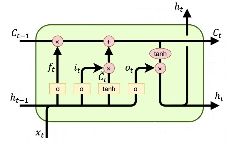
Figure 1: The structure of a unit in LSTM [9]

LSTM uses a gate mechanism to control the circulation and loss of characteristics, so in some degree, the long-term dependence can be eased. Its core part calls Cell Stat. That unit calculates how much information is retained and how much information is updated. Cell State can be expressed as

\( {c_{t}}={f_{t}}∗{c_{t−1}}+{i_{t}}∗{\widetilde{c}_{t}} \)

f_t is the forget gate. It stands for the characteristics of C_t-1 are used to calculate C_t. f_t is a vector with elements between [0, 1]. Generally, we take sigmoid as the activation function, and its output value is within [0, 1].

\( {i_{t}}=σ({W_{i}}\cdot [{ℎ_{t−1,}}{x_{t}}]+{b_{i}}) \)

\( {\widetilde{C}_{t}}=tanh{({W_{c}}\cdot [{ℎ_{t−1}},{x_{t}}]+{b_{c}})} \)

\( {\widetilde{C}_{t}} \) is the update value of cell state, obtained by the input data x_t and hidden nodes h_t-1 through the neural network layer. The activation function of C_t usually used tanh. i_t means input gate, which is used to control the features of C_t used to update \( {\widetilde{C}_{t}} \) , is also a vector with elements within [0, 1], calculated by the input data x_t and hidden nodes h_t-1 through the activation function sigmoid.

Finally, calculate the output of the hidden node h_t in order to compute the predicted value y_t and generate the complete input of the next time slice,

\( {o_{t}}=σ({W_{o}}[{ℎ_{t−1}},{x_{t}}]+{b_{o}}) \)

\( {ℎ_{t}}={o_{t}}∗tanh⁡({C_{t}}) \)

h_t is calculated by the output gate o_t and cell state C_t.

2.2. Bi-directional Long Short-term Memory (Bi-LSTM)

The difference between Bi-LSTM and LSTM is that the hidden layer of Bi-LSTM stores two layers, in which a reverse sequence is also took into account.

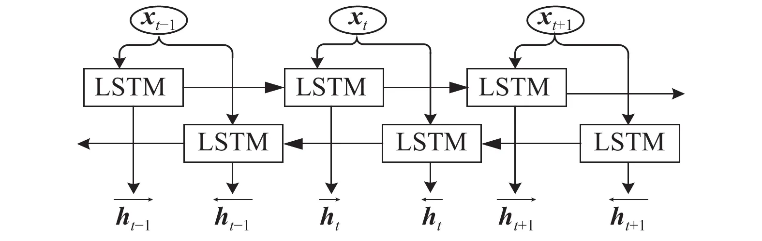
Figure 2: The structure of Bi-LSTM[10]

The calculation in forward layer is performed from time 1 to time t, and the output of the forward hidden layer at each time is obtained and saved while reverse calculation is performed in the backward layer from time t to time 1 to obtain and save the output of the backward hidden layer at each time as well. Finally, we combine the output of forward layer and backward layer at each time to get the Bi-LSTM output. Here are some equations:

\( {ℎ_{t}}=f({w_{1}}{x_{1}}+{w_{2}}{ℎ_{t−1}}) \)

\( ℎ_{t}^{ \prime }=f({w_{3}}{x_{t}}+{w_{5}}ℎ_{t−1}^{ \prime }) \)

\( {o_{t}}=g({w_{4}}{h_{t}}+{w_{6}}h_{t}^{ \prime } \) )

2.3. Stacked LSTM

The stacked LSTM consists of sevral LSTM layers. The upper LSTM structure outputs a sequence to the next LSTM structure instead of a single value. Adding depth in the LSTM layer is a more effective solution than adding memory cells within the LSTM unit. The basic structure of Stacked LSTM is shown below.

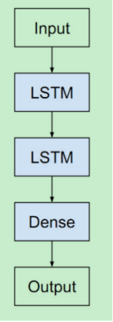
Figure 3: The structure of a Stacked LSTM[11]

3. Transformer

After word embedding and positional encoding, all words are converted into vectors. Then each word vector is multiplied by three matrices to get three new vectors in order to add more parameters to improve the model effect. The three vectors are query vector Q, key vector K and value vector V. For each word W, we use its Q to dot product the K of all input words. The result of dot product represents the similarity between the two words. Since the values have a large variance, resulting in unstable gradient, divide the results with the square root of the key vector’s length to make the gradient more stable. Using softmax function to normalize the fraction so that they are all positive and add up to 1. Multiply the value vector V by the results after softmax function to keep the values of the target words unchanged and cover up the irrelevant words. Add the weighted V vectors to generate the output of the self-attention layer of this position (the first word) and calculate the self-attention output of other positions in the same way.

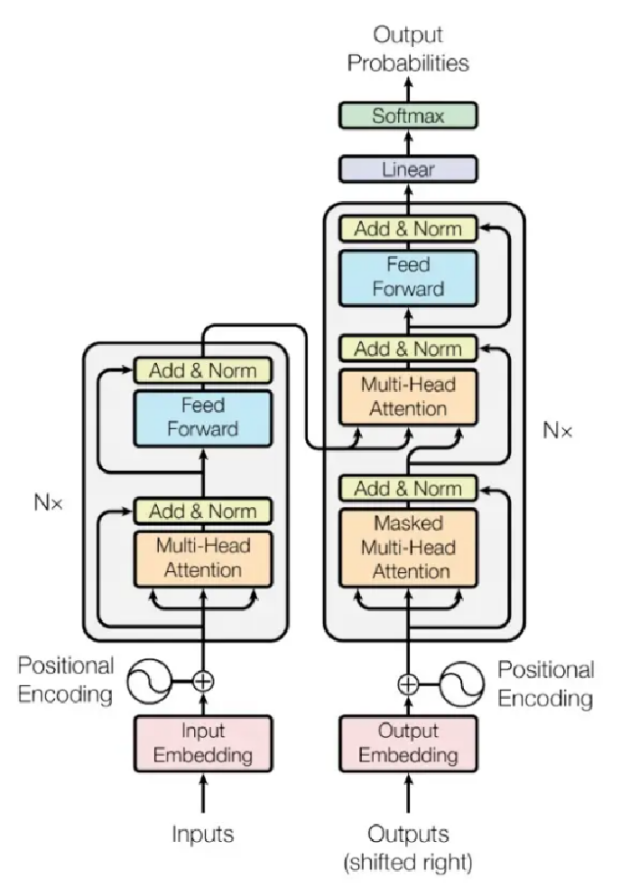
Figure 4: The structure of a Transformer[12]

In order to further refine the self-attention mechanism layer, use different Q/K/V matrices to calculate different weight matrices, each weight matrix is used to project input vectors into different representation subspaces. Then multiply a weight matrix with a matrix spliced with these matrices and get the output of self-attention layer with the same input size. Add the input and output vectors of self-attention layer and then normalize the result through the layer norm module and enter the feedforward neural network. Then use the add-norm method, and finally get another well-represented sequence structure.

4. METHODOLOGY

4.1. Stochastic Gradient Descent (SGD)

SGD is a simple but very effective method, which is often used to learn linear classifiers under convex loss functions such as logistic regression. Large-scale and sparse machine learning problems often encountered in text classification and natural language processing has successfully applied SGD.

Most of the time SGD is going towards the global minimum, while sometimes going away from the minimum, if the sample goes in the wrong direction. Therefore, SGD is noisy. On average, the result of SGD ends up going towards the minimum, but sometimes it's going in the wrong direction, since SGD never converges and always fluctuate around the minimum value. It is inefficient to process since it only trains one sample at a time.

4.2. Adaptive Gradient Algorithm (AdaGrad)

In the standard gradient descent method, each parameter uses the same learning rate in each iteration. Beacuse of the difference of convergence rate of each parameter in dimension, the learning rate is set according to the convergence of different parameters.

AdaGrad algorithm is learning from the idea of regularization, the learning rate of each parameter is adaptively adjusted in each iteration. In the 𝑡-th iteration, the cumulative value of the gradient square of each parameter is calculated first [13].

\( {G_{t}}=\sum _{τ=1}^{t}{g_{τ}}⨀{g_{τ}} \)

The parameter update difference of AdaGrad algorithm is

\( ∆{θ_{t}}=−\frac{α}{\sqrt[]{{G_{t}}+ϵ}}⊙{g_{t}} \)

While α is the learning rate, and ε is a very small constant set to maintain numerical stability, usually from e^-10 to e^-7.

In AdaGrad algorithm, if the accumulation of partial derivative of a parameter is large, its learning rate is relatively small. On the contrary, if its partial derivative accumulation is small, its learning rate is relatively large. However, as the number of iteration times increases, the learning rate gradually decreases.

The disadvantage of AdaGrad algorithm is that if the optimal point is still not found after a certain number of iterations, since the learning rate at this time is very small, it is difficult to continue to find the optimal advantage.

4.3. AdaDelta

AdaDelta algorithm (Zeiler, 2012) is an improvement of AdaGrad algorithm. Adadelta algorithm adjusts the learning rate by exponentially decaying the moving average of the square of the gradient. In addition, Adadelta algorithm also introduces the exponential decay moving average of parameter update difference Δθ of each time [14].

During the 𝑡 th iteration, the square of the moving average of exponential attenuation weight of the parameter updates difference Δθ is

\( ∆X_{t−1}^{2}=β∆X_{t−2}^{2}+(1−{β_{1}})∆{θ_{t−1}}⊙∆{θ_{t−1}} \)

β₁ is the attenuation rate. Since Δθ_t is unknown, it could only be calculated at ΔX_t-1.

The parameter update difference of AdaDelta algorithm is

\( ∆{θ_{t}}=−\frac{\sqrt[]{∆X_{t−1}^{2}+ϵ}}{\sqrt[]{{G_{t}}+ϵ}} \)

ΔX²_t-1 is the exponential decay moving average of parameter update difference Δθ.

4.4. Adaptive Moment Estimation Algorithm (Adam)

The Adam algorithm uses momentum as the parameter update direction and adaptively adjust the learning rate [15].

The Adam algorithm calculate the exponential weighted average of the gradient g²_t square and the exponential weighted average of the gradient g_t.

\( {M_{t}}={β_{1}}{M_{t−1}}+(1−{β_{1}}){g_{t}} \)

\( {G_{t}}={β_{2}}{G_{t−1}}+(1−{β_{2}}){g_{t}}⨀{g_{t}} \)

M_t is the mean of gradient, and G_t is the variance without subtracting the mean. Usually β₁ = 0.9, β₂ = 0.99.

If M₀ = 0 and G₀ = 0, then the value of M_t and G_t will be smaller than the true mean and variance at the beginning of the iteration, especially when β₁ and β₂ are all approach to 1. Therefore, it’s necessary to revise the deviation.

\( {\hat{M}_{t}}=\frac{{M_{t}}}{1−β_{1}^{t}} \)

\( {\hat{G}_{t}}=\frac{{G_{t}}}{1−β_{2}^{t}} \)

The parameter update difference of Adam algorithm is

\( Δ{θ_{t}}=−\frac{α}{\sqrt[]{{\hat{G}_{t}}+ϵ}}{\hat{M}_{t}} \)

The learning rate α = 0.001, and it could also be attenuated, for example,

\( {a_{t}}=\frac{{a_{0}}}{\sqrt[]{t}} \)

4.5. AdamW

In short, AdamW is the Adam optimizer plus L₂ regularization to restrict the parameter value from being too large [16]. Generally, when we add L2 regularization straightly to the loss function, the loss function will be

\( {L_{{l_{2}}}}(θ)=L(θ)+\frac{1}{2}γ{‖θ‖^{2}} \)

Therefore, when calculating g_t,

\( {g_{t}}←∇{f_{t}}({θ_{t−1}})+λ{θ_{t−1}} \)

For AdamW, the L₂ regularization adds on the calculation of θ_t

\( {θ_{t}}←{θ_{t−1}}−{η_{t}}(\frac{α{\hat{m}_{t}}}{\sqrt[]{{\hat{v}_{t}}+ϵ}}+λ{θ_{t−1}}) \)

5. EXPERIMENT

5.1. LSTM

Before we apply different models in our dataset, we checked the tweets, it contains some tags, links or @ signs. Those text can’t contribute to our sentiment classification tasks, so during pre-process, we removed the useless information. In the manual tagged dataset, there are five sentiment classifications. We counted the distribution of the classifications. Fortunately, both in the training and the test dataset, the numbers of quinary classifications are well balanced.

After the pre-process, we used the typical LSTM model with no changes, which didn’t perform good enough, we used pre-trained tokenizer RoBERTa. RoBERTa is a model trained from a large corpus. We counted the length of the tweets. The longest one contains 184 tokens. So, when the RoBERTa tokenizer encode the text, the max length attribute is limited in 200. Although LSTM is a pretty wise solution in NLP, for the covid tweets dataset, the accuracy can’t satisfy anyone. The exact probability is only 59.8%. The LSTM model can’t fit the dataset very good, so we looked through some variants of LSTM model. The most popular operations are Stacked-LSTM and Bidirectional LSTM. Will stacked structure help us improve the accuracy? Which depth is the best choice? In the chart below. We established the result of our experiment. The accuracy of the test dataset went up to 70.7% when we stacked another LSTM layer. It also helps in the next two additional LSTM layers, however the accuracy growth stopped in depth 5. It’s difficult to say whether 4 or 5 layers of LSTM is better. Considering the simple model will have less troubles. We believe that 4 layers of LSTM is good enough and proceeded our experiment.

Table 1. accuracy of stacked LSTM adjustment

Another intuitive way to improve accuracy is that we can combine the positive sequence and the negative sequence to capture the whole context. In that way, the depth of the network doesn’t change but the parameters doubled. We changed the network’s depth with both LSTM and Bi-LSTM structures. The result is that with the Bi-LSTM structure, the accuracy of depth 3 didn’t grow, but in depth 4 and depth 5, the accuracy grows a lot. So maybe that’s also a good idea to combine the sequences. But compared with the stacked model. The cost of bidirectional structure is also great, the parameters doubled, but the accuracy only grew 2 or 3 %. The stacking method adding another layer with one third or a quarter additional parameter can have the same effect.

Table 2. accuracy of Bi-LSTM adjustment

The SGD method always have the worst behavior, since it never converges and always fluctuate around the minimum value. From the analysis of the table, on average, the results of SGD go towards the minimum. AdaGrad and AdaDelta perform better in the test dataset, while the results of AdaDelta exceed 50%. The reason why AdaDelta algorithm has a better result than AdaGrad is probably because it adjusts the learning rate by exponentially decaying the moving average of the gradient square, while the learning rate of AdaGrad is fixed. It could be observed that Adam and AdamW with its variant have much better results among these optimizers, while with the increase of the epoch, AdamW becomes a better choice. AdamW is a combination of Adam and L₂ regularization, and it has the best results with the rising of epoch. We proceeded our experiment with this optimizer.

Table 3. accuracy of optimizer adjustment

Dropout is also a key method to the robust the model. When we back propagate the gradients, randomly stop the propagate process and the method will always strength our network. The dropout rate was also test in the network. The result is that 0.2 and 0.3 are both pretty good, that value is always used in similar research avoiding overfitting.

Table 4. accuracy of dropout adjustment

6. Transformer

For the NLP problems, transformer model is a newly proposed model. It consists of two main parts: the encoder part and the decoder part. Transformer uses three matrices to capture attention, so the relation between different parts of input corpus can be calculated and stored in a more mathematical format. Since transformer is a sequence to sequence (Seq2Seq) model, to use the complex model for sentiment classification, we only need to focus on the encoder part. Firstly, we used the pre-trained model “BERT-base-uncased” from Huggingface. The function BERTForSequenceClassification add a softmax layer for the classification tasks, so we can apply the model with finetuned parameters for the sentiment classification. Only one softmax layer is good enough. Compared with the LSTM models, which we have applied a lot of different structures and different optimizers and different parameters, the transformer model for classification only took 2 epochs to reach a stable and excellent accuracy—74.7%.

Only one softmax layer can lead to that outcome. Another finetune method is to train the training dataset on the pre-trained model to get our own model. So, the final classification model will consider the word distribution of our covid-19 tweets dataset. In our finetune experiment, we added [SEP] token at the end of all sentences and added [CLS] token at the beginning of all sentences. After that, we counted the max length of tokens. Like some tests reported, the MAX_LEN attribute affects the training speed significantly. For the training dataset, the max length of tokens is 226, that means we will pad or truncate the sentences to the same length. The base model is also “BERT-base-uncased”, a structure with 12-layer, 768-hidden, 12-heads, 110M parameters. The batch size was 32, learning rate was 2e-5, the number of epochs is 6, and the optimizer was AdamW, which always perform the best. Finally, we started the training process, we loaded the data into GPU and before each iteration, we reset the gradients. Within each epoch, the forward propagation and back propagation updated the parameters through the optimizer. Then we through the forward propagation process on the test dataset evaluated the loss and accuracy.

The accuracy of the first epoch is 80%, obviously a better outcome. During the next 3 epochs, the loss decreased, and the accuracy increased. But in the fifth and the sixth epoch, the loss and the accuracy on the test dataset stopped changing. The highest accuracy reached 85%, an excellent outcome. Finally, we got a finetuned model, it’s very time-consuming to train the big model, but the outcome is the best.

Table 5. loss and accuracy of transformer finetune

7. CONCLUSION

In our experiments, we finished the sentiment classification task for the covid-19 tweet dataset after data preprocessing. We mainly used the LSTM model with its variants and the transformer model. For this quinary classification task, the most basic single-layer unidirectional LSTM performed poorly on the dataset, so we considered the stacked LSTM model and the bidirectional LSTM model and the derived Transformer model. We compared the advantages and disadvantages between different models and adjusted our optimizer and adjusted the dropout values to prevent overfitting.

In the Transformer model, we first used a simple pre-training model "BERT-base-uncased" and added a softmax layer after the encoder part for the classification task. Although only a small change was made to the original model, we finally got a pretty good outcome. After that, we also finetuned the training data set for the model. In the original training data set of BERT, the training data corpus was very large, learning information from news media, tweets, and so on. We added training samples to the original model and finetuned it by adding the Twitter dataset and made simple modifications to the parameters of the original model. The accuracy on the test set reached 80% after only one epoch, and after training four epochs, the model stabilized, and the results were obtained with a final accuracy of 85%.

The impact of model selection on the outcome is significant when the strategy of model tuning is more reasonable, and small adjustments within the better interval of parameters do not significantly improve the results of the model. Although the existing transformer model has performed well, we note that different tokens have the same weight for the sentiment classification task, and the model does not focus too much on words with significant sentiment polarity such as terrible and excellent. The later expriment can improve the performance results of the whole model from the perspective of causal inference, such as using PSM to optimize the upstream task. And counterfactual inference of the sentiment polarity of each word by methods such as KNN and assigning its weight in the sentiment classification task accordingly would be a better boost. So far, no such study has been carried out due to time constraints, but in subsequent studies, we will consider causality and also continue to target improvements in models such as LSTM with added attention mechanisms for implementation.

Acknowledgement

Cai Wenyu and Liu Qizheng contributed equally to this work and are both second authors.

References

[1]. Galiatsatos, P. (2020, April 13). What Coronavirus Does to the Lungs. Www.hopkinsmedicine.org. https://www.hopkinsmedicine.org/health/conditions-and-diseases/coronavirus/what-coronavirus-does-to-the-lungs
[2]. Coronavirus tweets NLP - Text Classification. (n.d.). Www.kaggle.com. https://www.kaggle.com/datasets/datatattle/covid-19-nlp-text-classification
[3]. Schuster, Mike & Paliwal, Kuldip. (1997). Bidirectional recurrent neural networks. Signal Processing, IEEE Transactions on. 45. 2673 - 2681. 10.1109/78.650093.
[4]. S. Hochreiter and J. Schmidhuber, "Long Short-Term Memory," in Neural Computation, vol. 9, no. 8, pp. 1735-1780, 15 Nov. 1997, doi: 10.1162/neco.1997.9.8.1735.
[5]. Vaswani, A., Shazeer, N., Parmar, N., Uszkoreit, J., Brain, G., Research, G., Jones, L., Gomez, A., Kaiser, Ł., & Polosukhin, I. (2017). Attention Is All You Need. https://arxiv.org/pdf/1706.03762.pdf
[6]. Devlin, J., Chang, M.-W., Lee, K., & Toutanova, K. (2019). BERT: Pre-training of Deep Bidirectional Transformers for Language Understanding. ArXiv:1810.04805 [Cs].
[7]. Devlin, J., Chang, M.-W., Lee, K., & Toutanova, K. (2019). BERT: Pre-training of Deep Bidirectional Transformers for Language Understanding. ArXiv:1810.04805 [Cs]. https://arxiv.org/abs/1810.04805v2
[8]. Liu, Y., Ott, M., Goyal, N., Du, J., Joshi, M., Chen, D., Levy, O., Lewis, M., Zettlemoyer, L., & Stoyanov, V. (2019). RoBERTa: A Robustly Optimized BERT Pretraining Approach. ArXiv.org. https://arxiv.org/abs/1907.11692
[9]. MrDoghead. LSTM&Bi-LSTM[EB/OL]. https://blog.csdn.net/mch2869253130/article/details/89150043, 2021-04-19
[10]. Mathor. The application of BiLSTM with PyTorch[EB/OL]. https://wmathor.com/index.php/archives/1447/, 2020-06-28
[11]. Cskywit. [LSTM NOTE5]How to Develop Stacked LSTMs[EB/OL]. https://blog.csdn.net/cskywit/article/details/87460704, 2019-02-16
[12]. TensorFlow. Neural machine translation with a Transformer and Keras[EB/OL]. https://www.tensorflow.org/text/tutorials/transformer
[13]. Rosenbaum, Paul R.; Rubin, Donald B. (1983). "The Central Role of the Propensity Score in Observational Studies for Causal Effects". Biometrika. 70 (1): 41–55. doi:10.1093/biomet/70.1.41.
[14]. Duchi, J., Hazan, E., & Singer, Y. (2011). Adaptive subgradient methods for online learning and stochastic optimization. Journal of machine learning research, 12(7).
[15]. Kingma D, Ba J, 2015. Adam: A method for stochastic optimization[C]//Proceedings of International Conference on Learning Representations.
[16]. Loshchilov I, Hutter F. Decoupled weight decay regularization[J]. arXiv preprint arXiv:1711.05101, 2017.
[17]. Zeiler, M. (n.d.). ADADELTA: AN ADAPTIVE LEARNING RATE METHOD. https://arxiv.org/pdf/1212.5701.pdf
[18]. Kingma, D., & Lei Ba, J. (2017). ADAM: A METHOD FOR STOCHASTIC OPTIMIZATION. https://arxiv.org/pdf/1412.6980.pdf
[19]. Rui Chen, Jie Cao & Dan Zhang. "Probabilistic Prediction of Photovoltaic Power Using Bayesian Neural Network - LSTM Model", 2021 IEEE 4th International Conference on Renewable Energy and Power Engineering (REPE), 2021
Cite this article
Yang,H.;Cai,W.;Liu,Q. (2023). Sentiment Classification on tweets —Based on LSTM with variants and BERT finetune. Applied and Computational Engineering,6,1533-1543.
Data availability
The datasets used and/or analyzed during the current study will be available from the authors upon reasonable request.
Disclaimer/Publisher's Note
The statements, opinions and data contained in all publications are solely those of the individual author(s) and contributor(s) and not of EWA Publishing and/or the editor(s). EWA Publishing and/or the editor(s) disclaim responsibility for any injury to people or property resulting from any ideas, methods, instructions or products referred to in the content.
About volume
Volume title: Proceedings of the 3rd International Conference on Signal Processing and Machine Learning
© 2024 by the author(s). Licensee EWA Publishing, Oxford, UK. This article is an open access article distributed under the terms and
conditions of the Creative Commons Attribution (CC BY) license. Authors who
publish this series agree to the following terms:
1. Authors retain copyright and grant the series right of first publication with the work simultaneously licensed under a Creative Commons
Attribution License that allows others to share the work with an acknowledgment of the work's authorship and initial publication in this
series.
2. Authors are able to enter into separate, additional contractual arrangements for the non-exclusive distribution of the series's published
version of the work (e.g., post it to an institutional repository or publish it in a book), with an acknowledgment of its initial
publication in this series.
3. Authors are permitted and encouraged to post their work online (e.g., in institutional repositories or on their website) prior to and
during the submission process, as it can lead to productive exchanges, as well as earlier and greater citation of published work (See
Open access policy for details).