1. Introduction

Deep Q-Learning Network (DQN) is a deep reinforcement learning algorithm that combines Q-learning and deep neural network [1]. Since DQN algorithm can adopt high-dimensional state inputs and produce low-dimensional action outputs, it is frequently used to perform human-level control and even better than human, a common example is playing Atari games [2-3]. To optimize performance, some variants of DQN have been developed in the past ten years. However, appropriate tuning of hyperparameters is necessary for any variant, since hyperparameters control the actions of training algorithm directly and significantly affect the performance of deep RL models. At present, the relevant research is insufficient, so we conduct the experiment.

In this research, we compare the results from training with different hyperparameters such as number of episodes, size of replay buffer and gamma, then analyze how they affect the performance of the algorithm in the environment of OpenAI Gym’s CartPole-v1. CartPole-v1 is one of the most classic environments for reinforcement learning, it has maximum scores of 500 instead of 200 from the older version and only has simple actions to take which is informative for producing intuitive training results.

2. DQN

DQN is a reinforcement learning algorithm that combines Q-learning and deep neural network. As an improved version of Q-learning, DQN uses Q function Q(state, action | \( θ \) ) which is designed to approximate real Q(state, action), but originally it suffered from problems such as training is unstable and cumulative reward does not converge when deep neural network is applied [4]. Thus, the concept of using experience replay to train the agent was proposed. When training neural network without experience replay, it is usually assumed that data are distributed independently and identically, but data have strong correlation, instability of neural network can occur if these they are used for sequential training. However, experience replay can break the correlation between data effectively, as it allows agent to store learned data into a database with certain capacity and train its neural network by randomly taking samples from database.

The DQN updates the Q-function using the Bellman Equation:

Moreover, soft update is also applied to our DQN algorithm to ensure that the target network updates for every episode. More specifically, target network’s parameter \( θ_{i}^{-} \) uses current network’s parameter \( θ_{i} \) to update according to the following equation:

which can be simplified to:

where \( 0  \lt  ε ≪ 1 \) . By using soft update, DQN algorithm keeps stabilized, even though the target network updates for every episode. Similarly, as the soft update interval \( ε \) decreases, the stability increases, the speed of convergence decreases. Thus, an appropriate soft update interval \( ε \) makes training not only more stable but also faster. Our team sets \( ε = 0.005 \) as default value.

3. Experiments

3.1. Details

To conduct the experiment, we implemented a DQN algorithm and used CartPole-v1 from OpenAI Gym 0.15.7 as training environment. Compared to CartPole-v0, CartPole-v1 has higher maximum scores, which offers space for improved algorithms to present. Furthermore, we chose Python 3.8 and PyTorch 1.13.1 to build code because of better stability. CartPole is shown in Figure 1.

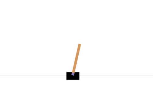
Figure 1. CartPole from Atari.

3.2. Performance comparison and analysis

3.2.1. Number of episodes. The number of episodes is a hyperparameter that determines how many times the DQN agent plays the game to train itself. Each episode consists of a sequence of states, actions, and rewards, and always ends with a terminal state. In our DQN algorithm, an episode ends if the pole falls, the cart reaches the edge, or the agent achieves a score of 500.

In supervised learning, a potential problem is overfitting, which occurs when a model learns the training data too well and performs poorly on new, unseen data. In deep reinforcement learning, overfitting can be a problem if the training environment is significantly different from the testing environment. However, since both environments in CartPole-v1 are the same, DQN algorithm should be well-fitted to the training data so that it can excel in this game [5].

In our experimental setup, we undertook the task of exploring the relationship between episodes and reward. Figure 2 depicts the outcome of this analysis, which also suggests that in the early stages of episode progression, the reward grows at a rapid pace and eventually stabilizes at later stages [6-7]. This pattern can be attributed to the fact that our network has been designed to learn from past experiences and continually improve its actions based on them.

As the network interacts with the environment and explores different scenarios, it gains a deeper understanding of the actions that lead to higher rewards and those that should be avoided. During the initial stages of training, the network may not have acquired sufficient knowledge to determine the optimal actions in every situation, which could result in lower rewards. However, as the network continues to learn and refine its actions and policy, its performance gradually improves, leading to higher rewards over time.

In summary, this experiment demonstrates that the network's ability to learn and adapt is a critical factor in maximizing the rewards it can achieve. By continuing to explore and refine its actions, the network can achieve optimal performance in a given environment.

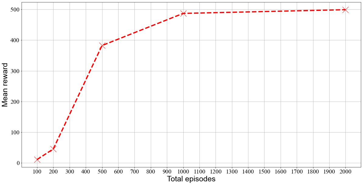
Figure 2. Mean Reward based on Total Number of Episodes.

3.2.2. Size of replay buffer. The replay buffer in a DQN network serves as a memory storage to store experience data generated from the agent's interaction with the environment. The replay buffer is then used to randomly select a subset of the stored experience data for training the DQN network. The primary functions of the replay buffer include reducing data correlation, improving data utilization efficiency, increasing sample diversity, relenting overfitting, and so on.

One of the primary advantages of using a replay buffer is that it reduces data correlation by removing temporal dependencies between consecutive samples. This allows for better utilization of data and prevents the DQN network from becoming biased towards certain types of experiences. Additionally, the replay buffer increases the diversity of samples by randomly selecting experiences, which helps prevent the DQN network from being stuck in local optima.

Another advantage of using a replay buffer is that it prevents overfitting by training the network on a random subset of the stored experience data rather than the entire dataset. This improves the generalization ability of the network and prevents it from memorizing the training data.

At the beginning, we set the size of replay buffer to 1000, and the agent didn’t perform well. As a result, we started to train the agent with larger replay buffer such as 5000, 10000, 20000, and 40000. Mean rewards for all training were recorded and used for comparison.

As shown in Figure 3, the reward increases as the replay buffer increases because more historical experience is stored to learn, and the agent can choose actions more accurately in a certain state to obtain greater rewards. However, when the replay buffer reaches a certain size, the reward tends to stabilize. This is because the historical experience in the replay buffer is sufficient enough for the agent to learn the environment, in which case, the learning effect on new experience is no longer significant. At this time, increasing the replay buffer does not significantly affect the network’s performance. An excessively large replay buffer will also bring storage and computational problems, leading to lower efficiency during training [8].

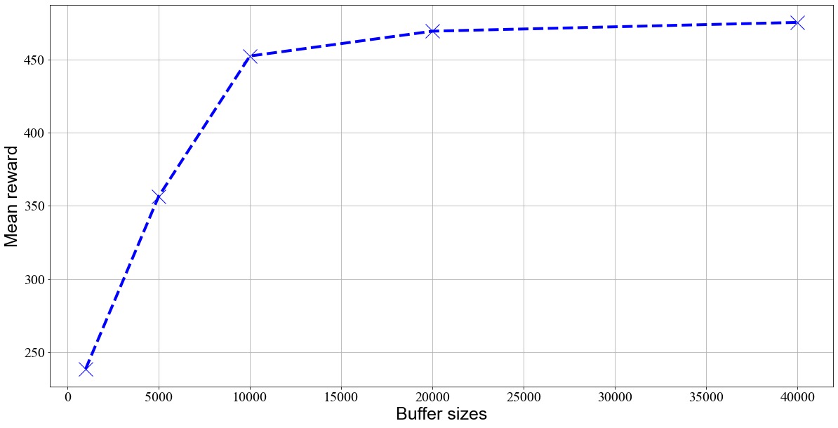
Figure 3. Mean Reward based on Buffer Size.

3.2.3. Gamma. In a DQN network, the γ value is a crucial hyperparameter that determines the trade-off between immediate and future rewards when validating an agent's performance. A higher γ value emphasizes future rewards, while a lower value emphasizes immediate rewards. Specifically, the γ value serves to discount future rewards, allowing the agent to balance the importance of immediate and short-term rewards against long-term rewards.

Typically, the γ value ranges from 0 to 1. When the γ value is close to 1, the agent gives greater weight to future rewards, which can lead to long-term planning and potentially better performance over the course of many steps. On the other hand, when the γ value is close to 0, the agent focuses more on immediate rewards, which may lead to a more reactive and opportunistic strategy. The discounted reward can be calculated by the following equation:

It is important to select an appropriate γ value based on the problem, as the optimal value may vary depending on the specific task or environment. Additionally, as the γ value increases, the agent may shift from being too focused on immediate rewards to being overly focused on future rewards, which may negatively impact training performance. Therefore, finding the right balance between immediate and long-term rewards is key to achieving optimal performance in a DQN network [9].

As depicted in figure 4, as the γ value increases, the mean reward generally increases, and the maximum reward is achieved at γ=0.97. However, when the γ value is too small, the agent may focus too much on immediate rewards, resulting in a short-sighted strategy that easily falls into local optimal solutions. As γ increases, the importance of long-term rewards is better accounted for, leading to a corresponding increase in the reward. However, there is a point where excessive emphasis on future rewards due to the large discount factor can lead to excessive exploration, resulting in poorer training performance [10]. Therefore, as the γ value continues to increase beyond this point, the reward will rapidly decrease. This experiment shows the importance of carefully selecting an appropriate γ value for the specific problem to achieve optimal training performance.

In terms of the magnitude of change, when the value of γ increases in the two intervals [0.9, 0.91] and [0.93, 0.97], the reward increases very quickly. When the γ value is between 0.91 and 0.93, although the reward also shows an increasing trend, the magnitude of increase is obviously not as large as in the other two intervals. However, when γ changes in the interval [0.97, 1.0], the reward declines rapidly at an equally fast rate. The experimental results in the interval [0.91, 093] should not differ so much from those in the other two intervals theoretically, suggesting that this may be related to the specific task environment.

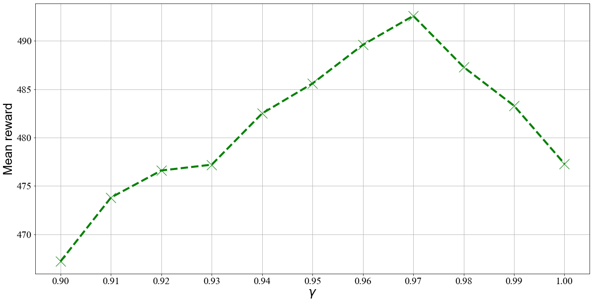
Figure 4. Mean Reward Based on Different Values of γ

3.2.4. Learning rate. Learning rate is a hyperparameter, acting like the stride length, to control the rate at which the algorithm learns and updates the parameters during the training process. If the learning rate is large, the model will be quickly modified in the beginning since each point is new to it. However, walking too fast means it may well ignore the minima and vibrate around it, thus being hard to converge. If learning rate is low, each step is too small to learn, so it will take longer time to descent and find the minimum value.

To better illustrate the performance, this paper used the concept of moving average reward, for example, average of the last hundred elements from rewards. Since the ADAM optimizer, which is an adaptive optimizer, is employed in our codes, we changed several values of its parameter, learning rate, including 0.00005, 0.0001, 0.0005. In figure 5, a comparatively high learning rate, 0.0005, seems to perform well at start with few samples, but as the problem becomes more complicated, the model fails to converge. By contrast, the learning rate of 0.00005 is too small to get a good outcome within 600 episodes. It is reasonable to assume a preferable learning rate is around 0.0001 in our DQN algorithm.

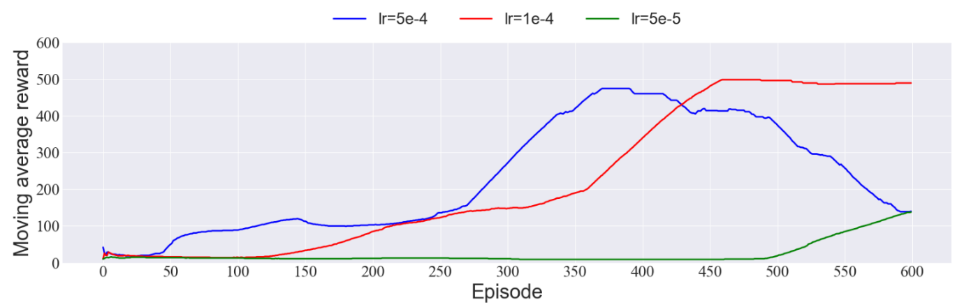
Figure 5. Comparison among the Moving Average Rewards of different Learning Rates.

Studies have found that even if ADAM optimizer is a kind of adaptive optimizer, some experiments show that adaptive approaches generalize more poorly than adaptive counterparts [6]. It may not be universally useful with problems with convergence to an optimal solution [4].

To study more about how learning rate affects DQN's performance, this paper also tests another strategy to adjust it. A common choice to manually adjust the learning rate is to decay it. The memorizing of noisy data is reduced by an initial high learning rate, while the acquisition of complex patterns is also enhanced by a subsequent declining learning rate [7]. In our algorithm, Cosine Annealing is employed to achieve that. However, figure 6 shows that it is not suitable to combine decaying learning rate with the ADAM optimizer in this algorithm. Researchers are advised to turn to some variant ADAM with long-term memory of previous gradients [4], or preferably, control the various parameters of the optimization iteration with a deeper understanding of the specific data and environment.

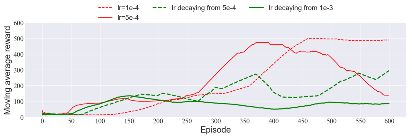
Figure 6. Comparison among the Moving Average Rewards of fixed Learning Rates and decaying Learning Rates.

3.2.5. Batch size. Batch size is the number of data samples captured in one training run. If the batch size is too small, it takes much time to train the model and potentially causes dramatic vibration. These updates need fewer calculations when the number of samples is modest. If the batch size is too large, different batches share similar gradient direction, thus easily falling into the local minima. However, with necessary dynamic adjustments, good generalization can be shown with big batches [1].

A method of updating this parameter with better performances in deep learning is to modify it proportionally to the quantity of data in Replay buffer [5]. The strategy can be transformed into the following equations:

Where k is the scale factor, len is the current size of replay, max is the max size of replay buffer and basicSize is a predetermined value from which the batch size starts to be adjusted.

We compared the performances of a model using a fixed batch size of 128 and a model with that of 256, as well as one with a dynamically adjusted batch size whose basic size is 128. In figure 7 we can see that, with fixed batch size of 128, the moving average reward fluctuates despite the initial rise, while the other two converge to nearly 500. Besides, compared with using a constant big batch size of 256, proportionally adjusting it from 128 to 256 lessens calculations in the beginning but offers good overall performance.

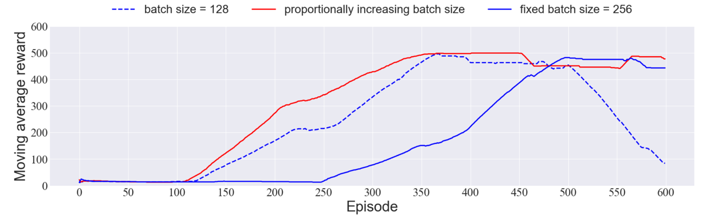
Figure 7. Comparison between Moving Average Rewards of fixed Batch Size and increasing Batch Size.

Furthermore, we compared several values of the basic batch size in figure 8, including 32, 64, 128, 256, 512. It demonstrates that 256 is a preferable choice in terms of basic batch size.

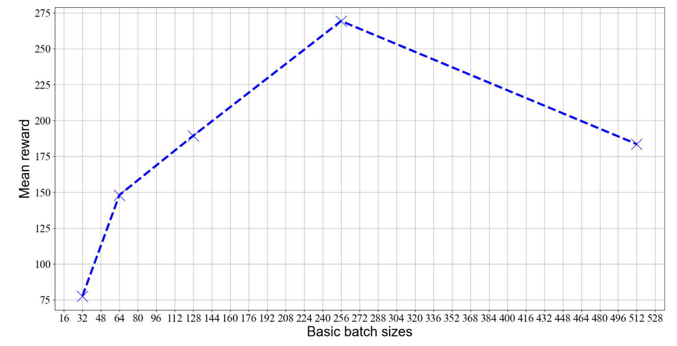
Figure 8. Mean Reward Based on Different Basic Batch Sizes.

4. Conclusion

This paper reconstructed the DQN algorithm codes according to previous work on classic DQN and soft updating. We trained it in the environment of CartPole-v1 with different hyperparameters and analyzed the performance. According to the testing results, the number of episodes and the size of replay buffer play important roles in the DQN algorithm. The more episodes, the better the performances. Expanding the replay buffer can contribute to the improvement until it exceeds 10000. In addition, gamma can improve our agent's performance most when its value is 0.97. In our environment, learning rate should not be too big or too small, a preferable choice being 0.0001, as decaying is of no necessity to be combined with the ADAM optimizer for better outcomes. What's more, the batch size is advised to be adjusted or increased in proportion to the current size of replay, where the basic size can be 256.

References

[1]. Hoffer, E., Hubara, I., & Soudry, D. Train longer, generalize better: closing the generalization gap in large batch training of neural networks. 2017 ArXiv (Cornell University). https://arxiv.org/pdf/1705.08741.pdf
[2]. Mnih, V., Kavukcuoglu, K., Silver, D., Graves, A., Antonoglou, I., Wierstra, D., & Riedmiller, M. Playing Atari with Deep Reinforcement Learning. 2013 Cornell University. http://cs.nyu.edu/~koray/publis/mnih-atari-2013.pdf
[3]. Mnih, V., Kavukcuoglu, K., Silver, D., Hassabis, D. Human-level control through deep reinforcement learning. 2015 Nature, 518(7540), 529–533.
[4]. Reddi, S. J., Kale, S., & Kumar, S. On the Convergence of Adam and Beyond. 2018 International Conference on Learning Representations 38(12) 233-244.
[5]. Smith, S. G., Kindermans, P., Ying, C., & Le, Q. V. Don’t decay the learning rate, increase the batch size. 2018 International Conference on Learning Representations. 312-324.
[6]. Wilson, A. C., Roelofs, R., Stern, M., Srebro, N., & Recht, B. The Marginal Value of Adaptive Gradient Methods in Machine Learning. 2017, Neural Information Processing Systems, 30, 4148–4158.
[7]. You, K., Long, M., Wang, J., & Jordan, M. I. How Does Learning Rate Decay Help Modern Neural Networks. 2019, ArXiv Cornell University. https://arxiv.org/pdf/1908.01878.pdf
[8]. Zhang, S., & Sutton, R.. A Deeper Look at Experience Replay. 2017 Cornell University. https://arxiv.org/pdf/1712.01275.pdf
[9]. Li H , Kumar N , Chen R , et al. Deep Reinforcement Learning. 2018 IEEE International Conference on Acoustics, Speech and Signal Processing,349-359.
[10]. Lillicrap T P, Hunt J J, Pritzel A et al. Continuous control with deep reinforcement learning. 2015 Computer science, 101-115.
Cite this article
Huang,Z.;Ou,J.;Wang,M. (2023). Comparison and analysis of DQN performance with different hyperparameters. Applied and Computational Engineering,15,22-29.
Data availability
The datasets used and/or analyzed during the current study will be available from the authors upon reasonable request.
Disclaimer/Publisher's Note
The statements, opinions and data contained in all publications are solely those of the individual author(s) and contributor(s) and not of EWA Publishing and/or the editor(s). EWA Publishing and/or the editor(s) disclaim responsibility for any injury to people or property resulting from any ideas, methods, instructions or products referred to in the content.
About volume
Volume title: Proceedings of the 5th International Conference on Computing and Data Science
© 2024 by the author(s). Licensee EWA Publishing, Oxford, UK. This article is an open access article distributed under the terms and
conditions of the Creative Commons Attribution (CC BY) license. Authors who
publish this series agree to the following terms:
1. Authors retain copyright and grant the series right of first publication with the work simultaneously licensed under a Creative Commons
Attribution License that allows others to share the work with an acknowledgment of the work's authorship and initial publication in this
series.
2. Authors are able to enter into separate, additional contractual arrangements for the non-exclusive distribution of the series's published
version of the work (e.g., post it to an institutional repository or publish it in a book), with an acknowledgment of its initial
publication in this series.
3. Authors are permitted and encouraged to post their work online (e.g., in institutional repositories or on their website) prior to and
during the submission process, as it can lead to productive exchanges, as well as earlier and greater citation of published work (See
Open access policy for details).