1. Introduction

In the past decade, modern convolutional neutral networks have accomplished numerous feats, ranging from image classification to autonomous driving. LeCun proposed the first modern model in 1990 by creatively applying the gradient back propagation algorithm to the training of a convolutional neural network in order to investigate the problem of handwritten identification [1]. This model broke the deep learning barrier and ushered in a new era of convolutional neural networks. The structure advocated by LeCun is known as Lenet, and it consists of the fundamental and fundamental elements that are extensively used in the deep learning field today, from the pooling layer to the fully connected layer. Research on deep learning continued to advance and reemerged as a popular topic in 2012.

Alex Krizhevesky and his collaborators from the University of Toronto presented a model in 2012 that was more extensive and comprehensive than LeNet. The 2012 ImageNet Large Scale Visual Recognition Challenge was won by the most effective model in the competition. The model employs ReLU as the activation function and dropout data augmentation to circumvent the overfitting issue [2]. The model is so effective that it revitalized the industry, and new models have emerged since then. Currently, the CNN family is more prosperous and is developing a variety of superb models and networks, including U-Net, YOLO, R-CNN, Fast CNN, etc. In this paper, the author intends to examine various extant model types, their brief operating principles, and a comparison of these models. It is hoped that the relevant research on deep learning and convolutional neural networks will be made available so that people can learn about the impact deep learning can have on human existence.

2. Convolutional neural network elements

2.1. Convolutional layer

The convolutional layer is responsible for the initial step of feature extraction and the majority of the computation. Convolution is used to aggregate all extracted information and generate a separate 2-dimensional matrix as a feature map. All neurons in the same feature map share the weight of the filter and the generated map, thereby reducing the network's complexity [3].

2.2. Stride

When researchers use CNN for image classification and feature extraction, they employ the convolution core depicted in figure 1. A stride is the number of node numbers a kernel shifts across the input matrix. Figure 1 depicts a 7*7 image and a 3*3 kernel core; if researchers wish to extract the data into the kernel, they must transfer the kernel core along the image. The kernel will output a 5x5 feature map in this manner. If the stride is modified from 1 to 2, a 3*3 output feature map is acquired.

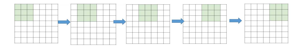
Figure 1. Stride 1, the filter window moves only one time for each connection [3].

To generalize this, the relationship between the output size and the convolutional core size is

\( O=1+\frac{N-F}{S} \) (1)

where O is for output map size, N is for input image size, and F is for convolutional core filter size, S is for the value of the stride [3].

2.3. Padding

Similar to edge detection in OpenCV, feature extraction also results in the loss of image border information. As depicted in Figure 2, when researchers implement a 5*5 feature map and a 3*3 convolutional core with a stride value of one, the kernel will be unable to access information beyond the border because there is no information beyond the border. To facilitate extraction, the algorithm fills empty nodes with the number zero, also known as zero-padding. It is permissible to include additional numbers on the border, but doing so it will introduce noise to the data and reduce the efficacy of the model and extraction.

By employing the buffering method, the original information of the image is preserved and the size of the feature map is maintained in accordance with the size of the original image. In addition, it can maintain the input of the deeper layer sufficiently informed.

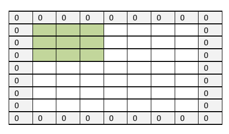
Figure 2. Zero-padding [3].

To generalize this, the relationship between the output size and the padding and the filter size is

\( O=1+\frac{N+2P-F}{S} \) (2)

where O is for output map size, N is for input image size, and F is for convolutional core filter size, S is for the value of the stride, P is the number of the layers of the zero-padding [3].

2.4. Pooling operation

After setting the padding and stride values, the filter has extracted sufficient data for processing. Theoretically, all the data extracted from the convolutional layer should be processed, but if the input image pixel is too large, the information processing pace will be slowed down. Therefore, researchers must continue to refine them and determine what the computer actually requires for feature extraction [4]. This procedure is known as merging operation. It not only preserves the essential characteristics but also reduces the extracted data size. It provides an alternative solution to the overfitting problem when fitting the model to the test set from the training set. It is a crucial stage in the feature extraction process. Current pooling types include Average Pooling, Max-Pooling Mixed Pooling, Pooling, and Stochastic Pooling, among others [5].

2.5. Fully connected layer and activation function

Before transferring the data to the neural network, the matrix must be flattened and the entirely connected layer must be formed. This operation reduces a two-dimensional matrix to a single dimension and functions as a classifier. It provides a method for discovering nonlinear relationships between the features and reduces the effect of data location.

Each node and layer in a neural network accepts information from the preceding layer and outputs it to the next layer. Without an activation function, it is more suitable for one-dimensional data processing. However, as the model advances to process higher dimension data, such as image classification, the information transferred from layer to layer will be linear, which is equivalent to a single hidden layer and makes the model more challenging to manipulate. By introducing activation function, nonlinear elements are introduced to the network to eliminate the disappearance of gradients after multiple network iterations [6]. CNN models frequently utilize Sigmoid, Tanh, softmax, and ReLU activation.

3. CNN model

The above part of paper presented a working process of convolutional neural network. In this part, the author presents a brief introduction model structures and features in sequence of LeNet, AlexNet, VGG (16) Net, GoogleNet, ResNet and DenseNet.

3.1. LeNet

In 1998, LeCun proposed Lenet, a convolutional neural network. Based on the MNIST data set, it was developed to identify the digits on a check. It is considered one of CNN's most significant networks in history [7]. People typically refer to the LeNet-5 model when discussing LeNet. It is comprised of 7 layers, including 3 convolutional layers, 2 subsampling layers, and 2 fully connected layers, and takes into consideration approximately 60000 parameters. It employs 22 average pooling, and the stride value is 2.

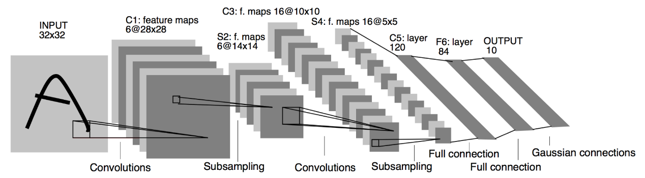
Figure 3. Lenet working principles [8].

3.2. AlexNet

AlexNet was created for the 2012 ImageNet Large-Scale Visual Recognition Challenge (ILSVRC). It was named after Alex Krizhevsky, the inventor of the network. The model claimed the competition's championship. AlexNet is more efficient than the competitor model. It was a defining moment that ushered in a period of accelerated growth in the study of deep learning.

Figure 4 illustrates the architecture of AlexNet. Three convolution layers and two entirely connected layers are present. AlexNet introduces Layer Normalisation and replaces tanh activation function with ReLU function in comparison to LeNet. This increases the speed by a factor of six, utterly obliterating the competition. Since then, the ReLU activation function has become standard in image classification tasks. In addition to the max pooling operation, AlexNet employs the dropout rate in the model to reduce the complexity of the data.

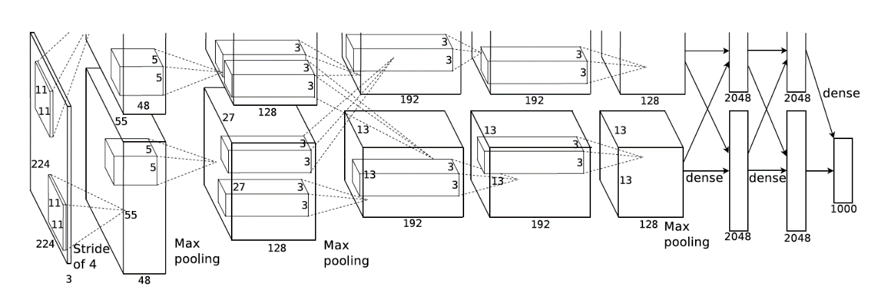
Figure 4. Structure of AlexNet [9].

3.3. VGG (16) Net

VGG stands for Visual Geometric Group, and the number 16 indicates the number of convolutional layers in the model. This network was published as part of the 2014 ILSVRC challenge. Even though it was the runner-up that year, it continues to be praised and widely accepted.

The model employs a filter with a 3*3 receptive field, and its convolution stride is 1. In the model, five max-pooling layers with a 2*2 pixel window conduct out the spatial pooling. As shown in figure 5, the model concludes with three fully connected (FC) layers. Each of the first two FC layers consists of 4096 channels, while the third FC layer consists of 1000 channels. Soft-max layer is the ultimate layer [10].

Unlike AlexNet, VGG(16)Net replaces the large kernel with 3*3 kernel and 1*1 kernel numbers. The benefit of this network is that it enhances the model's nonlinearity and makes the conclusion more convincing.

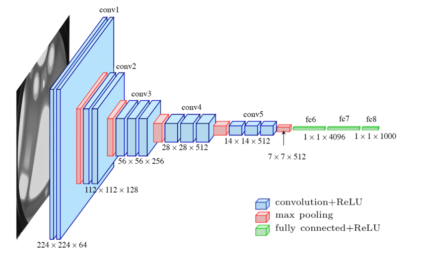
Figure 5. Structure of VGG (16) [11].

3.4. GoogleNet

Google's Christian Szegedi submitted GoogleNet, which won the 2014 ILSVRC, as the winning entry. It employs a 22-layer structure for a more robust network. It surpassed VGG Net in 2014 not only due to its more extensive network, but also due to the addition of "Inception Layers" to the network. There are a total of nine inception modules in the model, with filter sizes of 1X1, 3X3, and 5X5 determined by backpropagation effort. Before computing, these filters reduce the dimensionality. In addition, each module includes a maximum 3x3 pooling layer.

A further modification to GoogleNet is the replacement of all entirely connected layers with Global Average Pooling to calculate the average of each feature map. It aids in reducing the number of parameters and has no effect on the pace or precision.

3.5. ResNet

ResNet was created by Kaiming He in 2015, and it won the ImageNet 2015 challenge. It is an ultra-deep network with 152 layers that surpasses the human accuracy error rate of 3.6%, the lowest rate in the history of competition.

He utilized an enhanced version of ResNet: He used an arrangement of three layers, as opposed to the usual two, and designed the three layers to resemble a hamburger. The initial and final layers use 11 convolutions, while the intermediate layer uses 33 convolutions. The information entered the first layer and had its dimensionality reduced; consequently, the 33 filter will continue to reduce dimension and then elevate it back to its initial state. This structure made the model more effective.

3.6. DenseNet

DenseNet was published in CVPR 2017, consisting of multiple dense blocks and transition layers. It inherits the basic idea of RESNET, and establishes dense connections between all the layers, which is the reason that it was named after DenseNet. For a normal neural work, there will be number of L connections in the model if there are L layers. However, because of the unique architecture of the model, it has \( L(L+1)/2 \) connection. Figure 1 shows the connection mechanism of RESNET network. Benefiting from the structure, another advantage of DenseNet is feature reuse through the connection of features on the channel. These features enable Densenet to achieve better performance than RESNET with fewer parameters and computing costs and provide a solution for gradient vanishing.

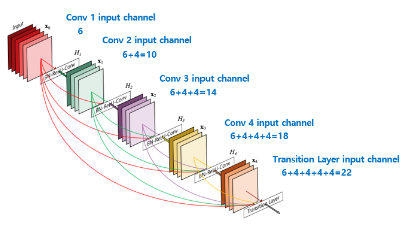
Figure 5. A 5-layer dense block with a growth rate of k=4 [12].

4. Conclusion

The author discussed the structure of a fundamental convolutional neural network in this paper. The convolutional layer requires the most computation and time, while the pooling layer and fully connected layer handle data processing and classification. LeNet proposed the network's fundamental architecture. AlexNet inaugurated the era of deep learning, while VGG-Net ResNet DenseNet propelled the deep learning field to its current prosperity. The enhancement of the models includes not only structural aspects but also efficiency. Researchers have made significant strides by modifying various parameters and enhancing the network in multiple versions. CNN continues to make contributions to fields such as computer version and robotics. This paper only provided a cursory analysis of how convolutional neural networks function and analyzed the characteristics of various CNN model types without presenting them in detail. In the future, the author will concentrate on optimizing the neural network model's structure and research methodology.

References

[1]. A. A. M. Al-Saffar, H. Tao and M. A. Talab, "Review of deep convolution neural network in image classification," 2017 International Conference on Radar, Antenna, Microwave, Electronics, and Telecommunications (ICRAMET), 2017, pp. 26-31, doi: 10.1109/ICRAMET.2017.8253139.
[2]. Krizhevsky A, Sutskever I, Hinton G E. Imagenet classification with deep convolutional neural networks[J]. Advances in neural information processing systems, 2012, 25: 1097-1105.
[3]. S. Albawi, T. A. Mohammed and S. Al-Zawi, "Understanding of a convolutional neural network," 2017 International Conference on Engineering and Technology (ICET), 2017, pp. 1-6, doi: 10.1109/ICEngTechnol.2017.8308186.
[4]. A. Ajit, K. Acharya and A. Samanta, "A Review of Convolutional Neural Networks," 2020 International Conference on Emerging Trends in Information Technology and Engineering (ic-ETITE), 2020, pp. 1-5, doi: 10.1109/ic-ETITE47903.2020.049.
[5]. Daneshgah Blvd., Shahrood, Iran,” Pooling Methods in Deep Neural Networks, a Review”
[6]. Athanasios Voulodimos , 1,2 Nikolaos Doulamis,2 Anastasios Doulamis,2 and Eftychios Protopapadakis ” Deep Learning for Computer Vision: A Brief Review”
[7]. Hao W, Yizhou W, Yaqin L, et al. The Role of Activation Function in CNN[C]//2020 2nd International Conference on Information Technology and Computer Application (ITCA). IEEE, 2020: 429-432.
[8]. LeCun Y, Bottou L, Bengio Y, et al. Gradient-based learning applied to document recognition[J]. Proceedings of the IEEE, 1998, 86(11): 2278-2324.
[9]. Krizhevsky A, Sutskever I, Hinton G E. Imagenet classification with deep convolutional neural networks[J]. Advances in neural information processing systems, 2012, 25: 1097-1105.
[10]. Simonyan K, Zisserman A. Very deep convolutional networks for large-scale image recognition[J]. arXiv preprint arXiv:1409.1556, 2014.
[11]. Max F, Ronay A. Automatic localization of casting defects with convolutional neural networks [J]. ResearchGate, 2017, 455.
[12]. Gao Huang, Zhuang Liu, Laurens van der Maaten, Kilian Q. Weinberger; Proceedings of the IEEE Conference on Computer Vision and Pattern Recognition (CVPR), 2017, pp. 4700-4708.
Cite this article
Wang,Z. (2023). Comparison of models of deep convolutional neural networks. Applied and Computational Engineering,16,50-55.
Data availability
The datasets used and/or analyzed during the current study will be available from the authors upon reasonable request.
Disclaimer/Publisher's Note
The statements, opinions and data contained in all publications are solely those of the individual author(s) and contributor(s) and not of EWA Publishing and/or the editor(s). EWA Publishing and/or the editor(s) disclaim responsibility for any injury to people or property resulting from any ideas, methods, instructions or products referred to in the content.
About volume
Volume title: Proceedings of the 5th International Conference on Computing and Data Science
© 2024 by the author(s). Licensee EWA Publishing, Oxford, UK. This article is an open access article distributed under the terms and
conditions of the Creative Commons Attribution (CC BY) license. Authors who
publish this series agree to the following terms:
1. Authors retain copyright and grant the series right of first publication with the work simultaneously licensed under a Creative Commons
Attribution License that allows others to share the work with an acknowledgment of the work's authorship and initial publication in this
series.
2. Authors are able to enter into separate, additional contractual arrangements for the non-exclusive distribution of the series's published
version of the work (e.g., post it to an institutional repository or publish it in a book), with an acknowledgment of its initial
publication in this series.
3. Authors are permitted and encouraged to post their work online (e.g., in institutional repositories or on their website) prior to and
during the submission process, as it can lead to productive exchanges, as well as earlier and greater citation of published work (See
Open access policy for details).