1. Introduction

At present, the more recognized mechanism of AD in the world is neuronal damage and synaptic loss caused by the deposition of neurofibrillary tangles and amyloid β-protein (Aβ) outside nerve cells. However, the specific pathogenesis of AD is not clearly defined because, once it appears, it will show an irreversible development trend. Therefore, if the diagnosis and appropriate intervention treatment can be made immediately in the initial stage of AD, it is likely to delay the progress of the disease. At present, relying only on manual analysis by physicians to process brain medical images is prevailing, which wastes time and energy. The use of artificial intelligence (AI) benefits physicians by helping them diagnose AD disease easily and quickly. The accurate diagnosis based on AI is helpful to achieve early intervention in the elderly, who are at high risk of disease, and improve their quality of life. So the author does research on deep learning based AI imaging probes for Alzheimer’s Disease. A model of densely connected network (DenseNet) as an AI technology, automatically learns the semantic features related to AD diagnosis on the brain MRI images from ADNI data. At the same time, for solving limited medical image samples problem, the effective transfer learning technology was applied in the experiment. The research in this article is beneficial for improving the diagnostic effectiveness of AD and its prodromal symptoms, and provides an advanced method for clinical diagnosis of AD on early stage aided by computers.

2. Literature review

Structural magnetic resonance imaging (sMRI) is commonly applied on the diagnosis of degenerative lesions in the brain, which tracks the brain structural changes and measures atrophy because of AD [1].

With the development of computer vision technology, deep learning methods, especially convolutional neural networks (CNN), have recently become a prevailing analytical method aided by computers.

In 2020, Li qingfeng, Xing xiaodan, and Feng qianjin from China Southern Medical University proposed an AI model of coupled convolutional and graph networks based on CNN diagnosis of AD. The experiment result shows the diagnosis accuracy reaching around 90% based on sufficient medical imaging data [2]. Mr. Shen Dinggang used the AI technology of two-stage task-oriented deep neural networks to locate the brain structures to distinguish the AD from NC accurately. The method achieved rapid feature point detection based on limited medical imaging [3].

Moreover, transfer learning is the tool of pre-trained models on different problems using smaller datasets. By adding relatively little data, which reduces a lot of training parameters, it shortens the training time, saves computing resources, improves the re-usability of the model, and avoids the overfitting of the model.In the experiment, the author studied the transfer learning framework, adopted DenseNet, one of the most advanced CNN architectures, pre-trained the model parameters with other medical image data, and then migrated them to AD and MCI data, which was used to classify the images into four categories: NC, sMCI, pMCI and AD. The main aim is to obtain precise results with limited data without overfitting. It overcomes the important problems in previous studies, such as less training data, weak model robustness and overfitting.

3. Data source and application methods

3.1. Data source and preprocessing

In the experiment, the medical image dataset MedMNIST is created by researchers as a pre-trained dataset for transfer learning [4].

At the same time, the world’s most famous public data set is adopted — AD Neuroimaging Program (The Alzhemer’s Disease Neuroimaging Initiative, ADNI) [5]. In the experiments, the data is related to MR-images in ADNI-1 and ADNI-2.

The dataset tested the presence of cognitive impairment by combining the Mini-Intelligence Status Examination Scale (Mini-mental State Examination, MMSE) and the Clinical dementia scale (Clinical Dementia Rating, CDR).

MMSE scores ranged from 20 to 26 points, and whose CDR score of 0.5 or 1 were labeled as being in the AD group [6][7]; subjects with a MMSE score of 24 to 30 and CDR score of 0, no depressive symptoms, no cognitive impairment, and no anxiety symptoms were labeled as being in the NC group [2]; Referring to the existing studies, the MCI subjects in the ADNI-1 and ADNI-2 datasets were further classified as sMCI (stable MCI) and pMCI (progressive MCI) according to whether the above subjects were converted to AD within 36 months after the first scan [8]. There were 229 NC, 199 AD, 167 pMCI and 226 sMCI subjects in the ADNI-1 dataset; 200 NC, 159 AD, 38 pMCI and 239 sMCI in the ADNI-2 dataset. It should be noted that the subjects appearing in the ADNI-1 and ADNI-2 datasets have been removed from the ADNI-2 dataset. Figure 1 shows example images of NC, MCI, MCI, and AD stages from ADNI-1 [5].

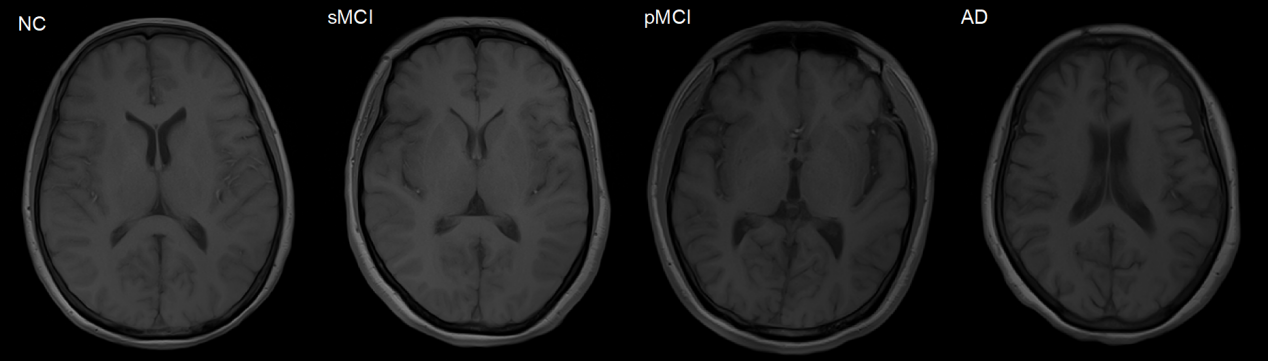
Figure 1. Example images from ADNI-1 [3].

The distribution of subjects in the above data sets is shown in Table 1.

Table 1. Distribution of subjects in the ADNI dataset.

To better evaluate the model, the ADNI-1 data is trained with and the ADNI-2 dataset is used as a separate test set. In particular, in ADNI-1, 20% of the data were randomly drawn as the validation set and others were used as the training set. The T1 sMRI data of all participants was processed by a set of standard pre-processing procedures, and each raw image was resampled normalized to 1×1×1 voxels and 256×256×256 images, followed by skull removal, image heterogeneous deviation correction, and finally by using the Colin27 template as a reference, each image was aligned to the same orientation [9].

To locate the brain sMRI, group comparisons were used to obtain the most statistical brain structures to differ the AD from NC groups. The method of rapid feature point detection is applied. Image blocks are obtained by taking the feature points after dithering as the center. Then the spatial location distribution of the 30 most differentiated brain feature point regions in the brain is marked.

3.2. DenseNet

Different from the natural image, because the brain nuclear magnetic image size is relatively large, during the training of convolutional neural network, different types of features in the image will include many subtle brain textures and changes in brain density, etc., and these primary feature information will be easily lost in the multi-layer convolutional operation, while the densely connected convolutional network (DenseNet) takes each layer’s feature map in the network as input to the other layers, which ensures that the primary features of the image are not lost with the deepening of the network layers. Thus, denseNet is proposed to complete the automatic diagnosis of AD diseases [10].

The specific dense connection blocks consist of several repeated compound functions \( {H_{l}}(∙) \) , the convolution layers of batch normalization, Relu and 3×3. The feature map size in the same in each dense block. The transition layer includes the batch normalization operation and an average pooling layer 2×2 for feature mapping for sampling the output of dense blocks, as shown in Figure 2.

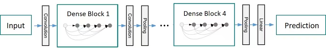
Figure 2. Structure diagram of DenseNet.

Due to the special connection mode of DenseNet, the feature graphs output will be larger, assuming that each composite function \( {H_{l}}(∙) \) generates k feature graphs, \( {k_{0}}+k×(l-1) \) input feature maps are on layer \( l \) . \( {k_{0}} \) is the number of input channels. That will make the entire network training process consume too much memory, time and other resources. To enhance the compactness of the model and also increase the computational efficiency, DenseNet takes two operations to reduce the feature graphs’ dimension. In the dense block, the \( 1×1 \) convolution layer is introduced before each compound function \( {H_{l}}(∙) \) to reduce the quantity of input feature maps, so that the composite function becomes: BN-ReLU-Conv ( \( 1×1 \) ) -BN-ReLU-Conv ( \( 3×3 \) ), reducing the number of feature maps output by each layer in the dense block.

For the transition layer, the convolution layer \( 1×1 \) is also introduced before the pooling layer, reducing the number of feature maps produced by the dense blocks, and the number of feature maps output by each dense block is halved. The initial convolution layer of the network is the \( 7×7 \) convolution layer with step size 2 and the largest pooling layer of \( 3×3 \) . The network finally contains a global pooling layer of \( 7×7 \) , and a fully connected layer.

3.3. Network transfer learning

CNN usually contain a large number of parameters, while medical image datasets are often relatively scarce, and the overfitting situation easily occurs when training deep network models with finite samples. In order to avoid the model overfitting, the network transfer learning strategy is adopted. It is based on DenseNet architecture, specifically before using network training ADNI data, using neural network for large medical image data set MedMNIST training, let the network learn medical image related characteristics and high-order semantic information. Later, the convolution layer of the denseNet is fine-adjusted using the ADNI dataset, and updates the layer’s parameters to complete the AD / NC diagnostic task and the pMCI / sMCI diagnostic task.

3.4. Deep learning language

This experiment was operated by Linux system. The deep learning framework is PyTorch, which is one of the current mainstream deep learning frameworks. The Python language is finally chosen to write the code for image pre-processing and model construction.

3.5. Parameter optimization and training of CNN network

Multiple adjustable sensitive parameters are included in the CNN, whose changes can affect the results of the experiment, so they need to be tuned in the experiment. The experiment tested the optimizer used in CNN, the size of the dropout probability value in the layer, the learning rate, Batch Size, and Epoch of the network then optimized the CNN. The network parameter settings of the final model are shown in Table 2.

Table 2. Setting of the parameters in experiment.

4. Experiments and results

To compare the method effectiveness here on the diagnostic task of AD and its prodromal disease, the diagnostic accuracy of denseNet combined with transfer learning is compared with that of three existing methods on the ADNI-2 dataset. The three methods are region of interest (ROI), voxel measurement (VBM), and full convolutional network model (wHFCN) based on prior information.

The pre-trained data uses the MedMNIST data. After training in advance, the ADNI data set is for optimizing the model. The convolution layer of the network is fine-tuned, the full connection layer is updated, and the problem of overfitting the network model is successfully solved. In the whole experiment, diagnostic accuracy, sensitivity, specificity, and area under the receiver operating characteristic curve (AUC) are compared respectively in the AD/NC diagnostic task and pMCI/sMCI diagnostic task.

The overall performance of the model is tested according to the loss curve and the subject operating characteristics (Receiver Operating Characteristic, ROC) curve (Figure 3), and the four more common evaluation measures, the area under the curve (Area Under Curve, AUC), sensitivity (Sensitivity, SEN), specificity (Specificity, SPE), and accuracy (Accuracy, ACC), are used to evaluate the performance of AD identification (Table 3). The formulas for SEN, SPC, and ACC are calculated as indicated, respectively.

\( SEN=\frac{TP}{TP+FN} \) (1)

\( SPC=\frac{TN}{TN+FP} \) (2)

\( ACC=\frac{TP+TN}{TP+FP+TN+FN} \) (3)

TP indicates the number predicted correctly from positive samples; FP represents the number predicted incorrectly from negative samples; TN indicates the number predicted correctly from negative samples; FN represents the number predicted incorrectly from positive samples.

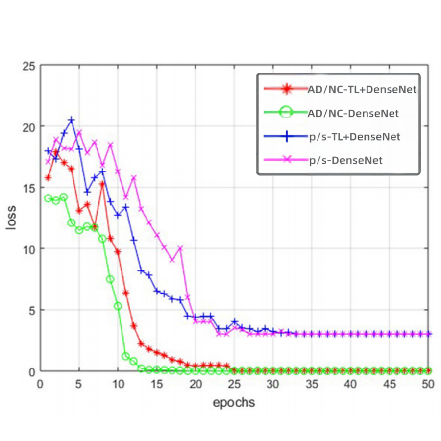
Figure 3. DenseNet and transfer learning + DenseNet loss curve.

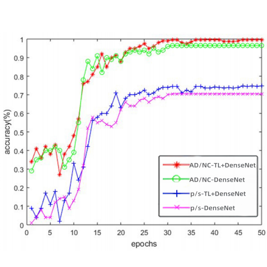
Figure 4. ROC curve in AD / NC diagnostic task and pMCI / sMCI diagnostic task.

The loss curve in Figure 3 illustrates that the difference between the predicted results of the two AI models (DenseNet coupled with transfer learning & pure DenseNet respectively) and the actual results gradually decreases to zero as the number of training increases. But it’s more important that the accuracy value of the model of DenseNet coupled with transfer learning in Figure 4 is faster to reach 100% in comparison with that of DenseNet alone.

Results from three existing methods in the literature ROI, VBM, and WH-FCN are used as the reference to verify the effect of the optimization model in AD discrimination experiments. Obviously, the results of diagnostic accuracy of the transfer learning + DenseNet model achieve the highest diagnostic accuracy of 90.8% both on the AD / NC and pMCI/sMCI diagnostic task, as well as the maximum AUC value, as shown in Table 3 in comparison with 3 existing methods.

Table 3. Test results of the different methods in the AD / NC diagnostic task- task 1and the pMCI / sMCI diagnostic task-task 2.

The comparative experimental results on the ADNI-2 data set suggest that the three methods based on deep learning (wH-FCN, DenseNet, transfer learning + DenseNet) are significantly better than the two methods (ROI and VBM + DenseNet) based on traditional machine learning for the diagnostic task of AD and its precursors. On both diagnostic tasks, the proposed method has significantly improved the classification performance compared to only using the dense connection network method. For AD/NC diagnostic tasks, in comparison to the existing methods, the optimized method gains better achievements, including the highest ACC and AUC. In the pMCI / sMCI diagnostic task, its performance is also excellent, and the gap between ACC, SEN, and SPE is within 0.1, and AUC is the highest value.

In summary, the performance of the model of DenseNet coupled with transfer learning is not only more accurate than the model of pure DenseNet but also better than that of the three existing methods of ROI, VBM, and WH-FCN on AUC, sensitivity, specificity, and accuracy.

5. Discussion

The method presented in this paper aims to predict disease labels without considering the intrinsic association between other factors (e.g., age, sex, MMSE, CDR-SB, etc.) and disease labels. As a feasible scenario, in the future, it is expected to embed a multi-task strategy in the model structure to adaptively learn the relationship between other factors and the disease labels. Provide a way to further improve the accuracy and stability of disease label prediction tasks.

Meanwhile, although the proposed method in this thesis has achieved high classification accuracy in the diagnosis of Alzheimer’s disease, the samples are limited corresponding to the ADNI public dataset. Due to the deficiencies such as single population, single mode, etc. in this data set, several problems are not clear and deserve further study in the future. For example, 1) Single group problem: whether the model trained on a specific data set or group can be promoted or transferred to other data sets/groups. Because this study is based on a North American model of Alzheimer’s disease diagnosis, whether it can be well predicted in Asian populations has not been explored; 2) Unimodal problem: Generally speaking, multi-modal neuroimaging data performance is better in terms of the diagnostic accuracy of AD than unimodal data. Considering Alzheimer’s disease and its precursor symptoms are associated with a variety of physiological indicators such as sugar metabolism and brain function connections, and T1 sMRI data mainly provides the structure of the brain information, adding other imaging modalities, such as resting-state functional magnetic resonance imaging and positron emission computed tomography imaging, can provide more information for disease diagnosis. This method is called multi-modal fusion, which can further improve the diagnostic accuracy and stability.

6. Conclusion

Compared with traditional feature extraction methods, as an adaptive feature extraction method, deep learning can hierarchically extract and integrate features from the original data space so as to obtain a better feature representation for the target task. The transfer learning + dense connection network method not only finds a way that the rare medical image data can easily lead to model overfitting but also works out that the medical image scale is large and easy to lose subtle primary features in training. The results show that Dense+transfer learning model can improve the diagnostic effect of AD and its prodromal symptoms and has good stability. It provides a new method for the clinical realization of the diagnosis of AD at early stage aided by computers.

Acknowledgment

Firstly, I would like to give my sincere and hearty gratitude to my teacher in school who gave me kind encouragement and useful instruction during the preparation of this thesis. In addition, many thanks extend to my family for their love and support. Finally, I am really grateful to all those who devote much time to reading this thesis and putting forward suggestions, which will benefit me in my later study.

References

[1]. Frisoni, Giovanni B., et al. 2010. “The clinical use of structural MRI in Alzheimer disease.” Nature Reviews Neurology 6.2: 67-77.
[2]. Li Qingfeng, Xing Xiaodan, Feng Qianjin. 2020. The magnetic resonance diagnosis method of Alzheimer’s disease based on the coupled convolution-graph convolutional neural network [J]. Journal of Southern Medical University, 40 (4): 7.
[3]. Zhang, Jun, Mingxia Liu, and Dinggang Shen. 2019. “Detecting anatomical landmarks from limited medical imaging data using two-stage task-oriented deep neural networks.” IEEE Transactions on Image Processing 26.10: 4753-4764.
[4]. Yang, Jiancheng, Rui Shi, and Bingbing Ni. 2021. “Medmnist classification decathlon: A lightweight automl benchmark for medical image analysis.” 2021 IEEE 18th International Symposium on Biomedical Imaging (ISBI). IEEE.
[5]. Jack Jr, Clifford R., et al. 2008. “The Alzheimer’s disease neuroimaging initiative (ADNI): MRI methods.” Journal of Magnetic Resonance Imaging: An Official Journal of the International Society for Magnetic Resonance in Medicine 27.4: 685-691.
[6]. Chapman K R, Bing-Canar H, Alosco M L, et al. 2016. Mini Mental State Examination and Logical Memory scores for entry into Alzheimer’s disease trials [J]. Alzheimer’s research & therapy, 8(1): 1-11.
[7]. O’Bryant , Sid E., et al. 2010. “Validation of the new interpretive guidelines for the clinical dementia rating scale sum of boxes score in the national Alzheimer’s coordinating center database.” Archives of neurology 67.6: 746-749.
[8]. Liu, Mingxia, et al. 2018. “Joint classification and regression via deep multi-task multi-channel learning for Alzheimer’s disease diagnosis.” IEEE Transactions on Biomedical Engineering 66.5: 1195-1206.
[9]. Holmes, Colin J., et al. 1998. “Enhancement of MR images using registration for signal averaging.” Journal of computer assisted tomography 22.2: 324-333.
[10]. Huang G, Liu Z, Laurens V, et al. 2016. Densely Connected Convolutional Networks [C]// IEEE Computer Society. IEEE Computer Society.
Cite this article
Ji,Y. (2023). Deep learning-based artificial intelligence imaging probes for Alzheimer’s disease. Applied and Computational Engineering,17,1-9.
Data availability
The datasets used and/or analyzed during the current study will be available from the authors upon reasonable request.
Disclaimer/Publisher's Note
The statements, opinions and data contained in all publications are solely those of the individual author(s) and contributor(s) and not of EWA Publishing and/or the editor(s). EWA Publishing and/or the editor(s) disclaim responsibility for any injury to people or property resulting from any ideas, methods, instructions or products referred to in the content.
About volume
Volume title: Proceedings of the 5th International Conference on Computing and Data Science
© 2024 by the author(s). Licensee EWA Publishing, Oxford, UK. This article is an open access article distributed under the terms and
conditions of the Creative Commons Attribution (CC BY) license. Authors who
publish this series agree to the following terms:
1. Authors retain copyright and grant the series right of first publication with the work simultaneously licensed under a Creative Commons
Attribution License that allows others to share the work with an acknowledgment of the work's authorship and initial publication in this
series.
2. Authors are able to enter into separate, additional contractual arrangements for the non-exclusive distribution of the series's published
version of the work (e.g., post it to an institutional repository or publish it in a book), with an acknowledgment of its initial
publication in this series.
3. Authors are permitted and encouraged to post their work online (e.g., in institutional repositories or on their website) prior to and
during the submission process, as it can lead to productive exchanges, as well as earlier and greater citation of published work (See
Open access policy for details).