1. Introduction

Galaxies represent massive systems encompassing stellar remnants, interstellar gases, stars, dust and dark matter bound together by gravity [1]. These cosmic entities exhibit a non-uniform spatial distribution, exhibiting considerable variations in terms of diameter and morphological structure. In recent years, large-scale photometric surveys across a wide range of wavelengths have produced great quantities of image data of galaxies using various telescopes. For example, the Dark Energy Camera on Blanco 4m telescope is highly sensitive and has a wide area of view, making it a perfect choice for obtaining photometry in the g, r and z bands.

In the large-scale study of the universe, classifying galaxies based on their visual morphology is the initial stage towards a better understanding of galaxy formation and evolution. The pivotal milestone in this endeavour can be traced back to Edwin Hubble’s seminal work in 1926, wherein he proposed a classification system based on the shape of galaxies as observed at optical wavelengths from earth, and since then, more and more intricate classification systems have been developed by researchers over time [2]. However, the earliest approaches employed for categorizing galaxies in various classes is to classify galaxy images manually, resulting in inconsistent standards and lack of efficiency when dealing with large volumes of data. In the past 30 years, machine learning algorithms have emerged as a pivotal tool in the classification of galaxies [3]. Although these methods can automatically classify a large number of data efficiently, most of them are based on analysing physical parameters of the galaxies, which requires complex feature engineering and solid background knowledge. Hence, researchers have turned their sights to deep learning algorithms, which can utilize massive amount of image data to find automated metrics that reproduce the probability distributions derived from human classifications.

Over the past decade, studies in deep learning have experienced remarkable advancements with new applications across diverse domains including the healthcare, finance, and many other industries. Deep learning models composed of multiple layers can approximate almost any non-linear functions either for regression tasks or classification tasks. For image classification, convolutional neural network (CNN) has become a commonly used approach owing to its efficiency. With the increasing availability of large datasets of galaxy image, some studies on classifying galaxies with CNN have yielded good results. For instance, Dieleman et al. developed a CNN with 7 layers for Galaxy Zoo Challenge and obtained the highest accuracy in 2015 [4]. In 2017, Aniyan and Thorat proposed TOOTHLESS, which is the first CNN to classify radio galaxies based on morphological feature [5]. Zhu et al. propose a modified Residual Network (ResNet) to classify galaxies into 5 classes using Galaxy Zoo dataset [6]. In 2021, Burger Becker et al. compared the performance of several CNNs for radio galaxy morphological classification on multiple metrics [7]. Since then, several new CNNs have been developed using transfer learning to classify galaxies [8].

Typically, a CNN consists of a feature network composed of convolutional layers and a task network composed of dense layers. Although previous studies have achieved satisfactory performance on respective datasets, most of these CNNs focus solely on the structures of the convolutional layers and only use an average pooling layer followed by an output layer as the final dense layers. A study on these CNNs has reported that models overfit quickly when training on a small dataset [7]. However, a similar study on automatic modulation classification has reported that by adding dropout after the dense layer, the classification results are better than the previous network, with higher convergence rate, faster training speed, and more balanced validation performance across categories [9].

In this regard, this paper investigated how different dropout rates of four types of fully connected layers can affect the overall performance of two types of CNNs on galaxy classification. It used 17,736 images of galaxy form the Galaxy10 DECaLS dataset, and performed four forms of data augmentation to reduce overfitting. The convolutional layers of models were chosen from 2 light-weighted models: the EfficientNetB0 and DenseNet121. These models utilize pertained weights from ImageNet as the initial weights. The dropout rates of each dropout layer were set to 0%, 10%, 20%, 30%, 40%, 50%, 60%, 70%, 80%, and 90%. Furthermore, after comparing model performances, to understand what the CNNs learn, this paper produces salience maps and Grad-CAM to provide qualitative analysis.

2. Method

2.1. Dataset description and preprocessing

This paper utilized the Galaxy10 DECaLS dataset released by Galaxy Zoo, which is a much-improved version of the original Galaxy10 dataset [10]. It contains 17,736 256×256 pixels coloured galaxy images (g, r and z bands) separated in 10 classes using volunteer votes. Figure 1 displays several images of each class from the Galaxy10 DECaLS dataset. However, as shown in Figure 2, the Galaxy10 DECaLS dataset is highly imbalanced between classes. The class Cigar Shaped Smooth Galaxies has only 334 images, which approximately accounts for 1.88% of the total samples.

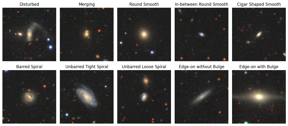
Figure 1. Example images of each class from the Galaxy10 DECaLS dataset.

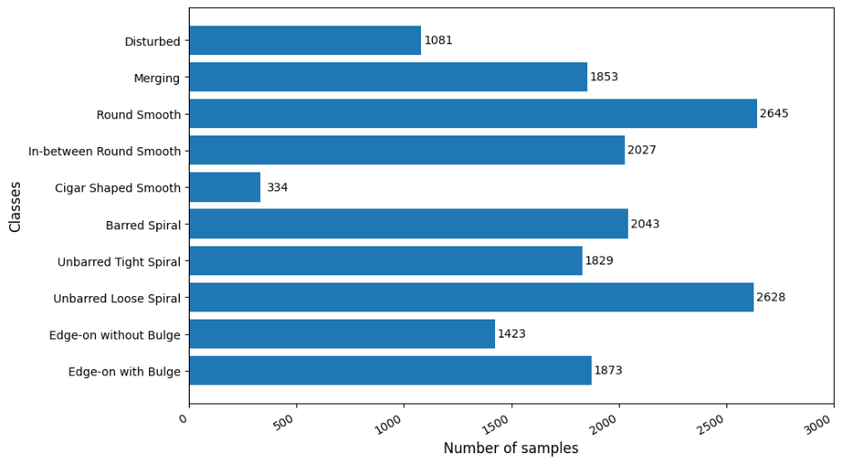
Figure 2. Samples distribution of classes from the Galaxy10 DECaLS dataset.

In terms of preprocessing, this paper first standardized the image feature-wise using mean and standard deviation of the dataset. Standardization of input data has been proven to be effective in speeding up model convergence and increasing classification accuracy. Then, the image was resized from 256×256 pixels to 224×224 pixels, which is the input dimension for CNNs pre-trained on the ImageNet dataset. Subsequently, a Morphological Opening was performed to eliminate noise that scattered around the centre of the image and to focus more on the morphological characteristics of galaxies. Morphological Opening is a variant form of two basic morphological operators, which involves performing an erosion operation followed by a dilation operation [11].

Data augmentation is commonly used to prevent overfitting. Therefore, for training and validation data, this paper utilized 3 types of data augmentation procedure including random rotation, random magnification, and random flipping. During these procedures, to avoid adding more noise to the input, points outside the boundaries was filled with a constant value of 0. Figure 3 shows some images before and after data augmentation and preprocessing.

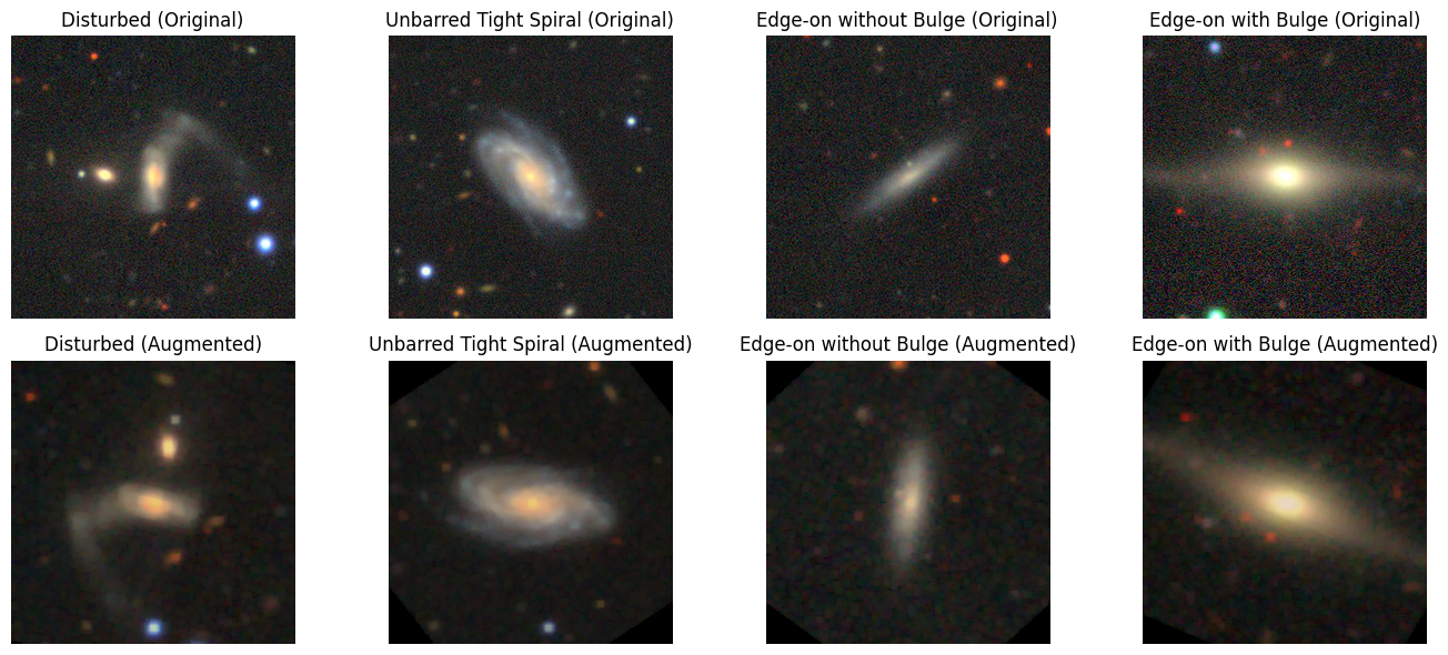
Figure 3. Example images before and after data augmentation and preprocessing.

2.2. CNN-based galaxy classification model

Convolutional neural network is a prominent variant of artificial neural network extensively employed in deep learning [12]. It is widely used for computer vision application [13-15], and is highly efficient for automatic image feature extraction. A typical CNN consists of a feature network with several convolutional layers and pooling layers, followed by a flatten layer to convert multi-dimensional tensor into a single dimensional tensor, and some fully connected layers to provide prediction results based on the extracted features.

The convolutional layers use filters composed of kernels, which are matrixes of learnable weights, to process the input and generate feature maps. Then, a non-linear function, usually ReLU, is used for activation. The utilization of kernels introduces translational invariance and parameter sharing to traditional neural networks. Generally, each convolutional layer learns features of increasing complexity. Thus, CNNs learn features in a hierarchical way. The pooling layers are often used after convolutional layers to reduce data sizes. They are invariant to small local transitions and has no learnable parameters. Max pooling and average pooling are two common choices for pooling layers. They take the maximum and the average value, respectively, within a sliding window of pixels.

The DenseNet and EfficientNet are two variants of typical CNNs. As illustrated in Figure 4, the DenseNet concatenates the output feature maps of the layer with the incoming feature maps within a dense block [16]. This method provides the network with maximum gradient and information flow, and resolves the issue of vanishing gradient. As for the EfficientNet, it was originally designed using neural architecture search in 2019 [17]. It introduces method called compound scaling, which balances the width, depth, and image resolution of the network against the available resources to improve its overall performance. Particularly, the baseline network EfficientNetB0 was obtained by performing a grid search on 3 dimensions of the network using AutoML [18]. Figure 5 shows the architecture of the EfficientNetB0.

This paper applied transfer learning to the DenseNet121 and EfficientNetB0, both of which utilized pretrained weights from ImageNet as the initial weights. These weights were set to trainable, since the galaxies images were quite different from the ImageNet data. In the context of galaxy classification, the fully connected layers for these CNNs were modified. Global average pooling layer and flatten layer were added after the last convolutional layer to convert input dimensions. A final dense layer with 10 neurons and SoftMax activation were used for classification. To investigate the effects of different dropout rates on models’ overall performance, various combinations of dropout layers and dense layers were added between the GAP layer or flatten layer and the final dense layer. Details about the abovementioned models are depicted in Table 1.

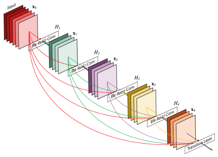
Figure 4. Architecture of a dense block within the DenseNet [16].

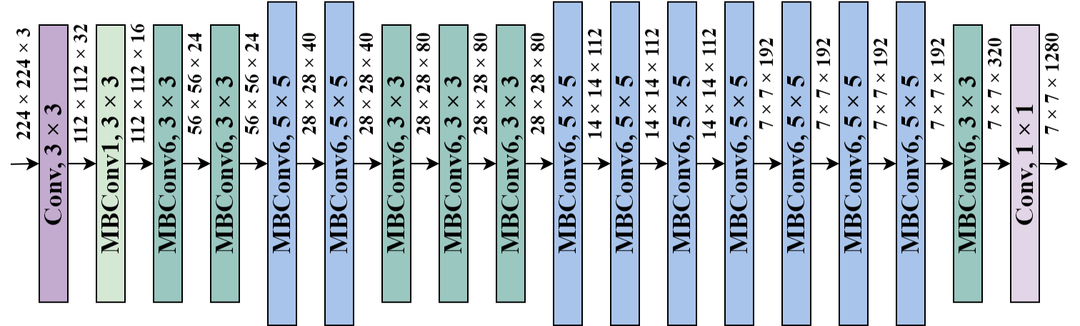
Figure 5. Architecture of the EfficientNetB0 [17].

2.3. Implementation details

This implementation is mainly based on TensorFlow, and models were trained with an NVIDIA RTX4090 GPU. For this experiment, the original dataset was divided into train, validation, and test sets in the ratio of 65:15:20 for ensuring that models can be better compared and validated in unbiased situations. For training, models used standard categorical cross-entropy as loss function, and Adam was used as the optimizer with a batch size of 64, a Nesterov momentum of 0.9, and a RMSProp ratio of 0.99. During training, the learning rate was modified before every epoch, and it followed a schedule of Exponential Decay with an initial value of 0.001 and a decay rate of 0.1. To deal with the imbalanced training data, class weights were used to force the models to learn more from the data from minority classes. The training process stopped after maximum 60 epochs, and it also utilized early stopping technic with a patience of 45 epochs to monitor validation accuracy.

3. Results and discussion

3.1. Classification performance

This paper conducted an extensive training process involving a total of 80 models, which can be divided into 8 different architectures as depicted in Table 1. For each architecture, 10 models were trained with a dropout rate of 0%, 10%, 20%, 30%, 40%, 50%, 60%, 70%, 80%, and 90%, respectively. Due to the excessive number of models trained in the experiment, only the results of CNNs with the highest validation accuracy for each architecture are shown in Table 2, and Figure 6 shows the corresponding training accuracy curve for these models. As shown in Figure 6, most of these models converged after training for 40 epochs, and their training accuracy improved smoothly, resulting from the learning rate schedule of Exponential Decay during the training process.

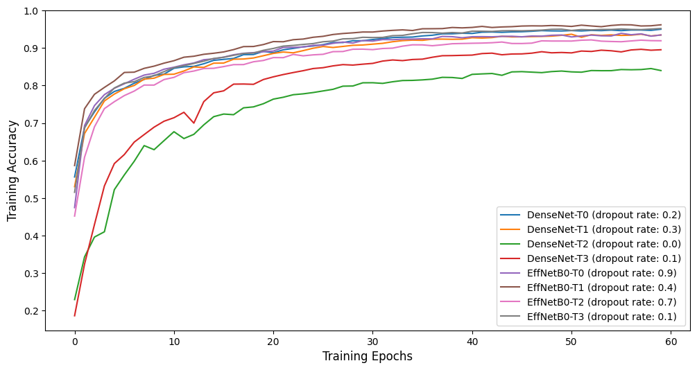
Figure 6. Training accuracy curve for the CNNs in Table 2.

As presented in Table 2, the DenseNet-T1 with a dropout rate of 0.3 obtained the best performance at the 31th epoch, with an accuracy of 87.14% on validation set. For test dataset, this model achieved an overall accuracy of 85.23%, and the details of its performance for each class are shown in Table 3. Although the dataset is highly imbalanced between classes, the performance for each class is relatively balanced. The class Cigar Shaped Smooth Galaxies, which has the least amount of data, still has an F1-score of 79.47%. This is attributed to the utilization of class weights, which improved the efficiency of learning from imbalanced data during the training process.

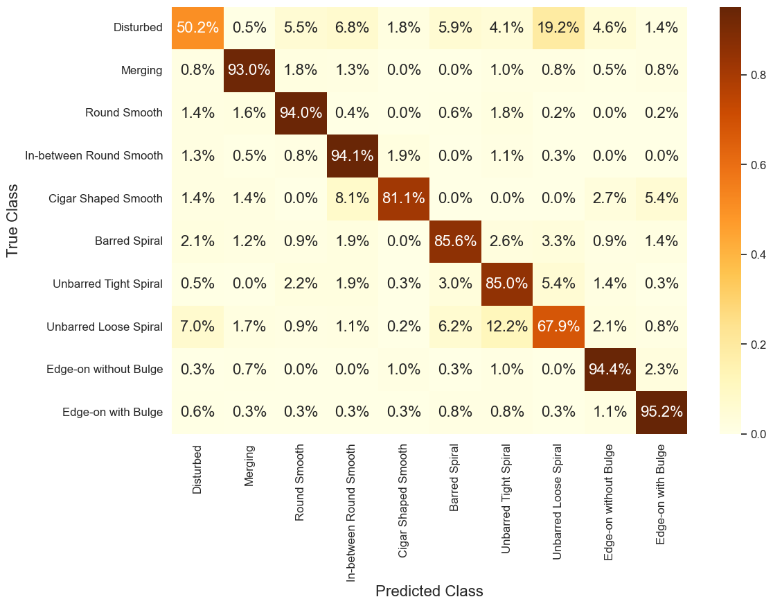
Figure 7. Confusion matrix of the DenseNet-T1 (dropout rate 0.3) on test set. The percentage given in each square is the normalized value for each class.

However, this model tends to confuse classes Disturbed Galaxies and Unbarred Loose Spiral Galaxies, according to the confusion matrix shown in Figure 7. To interpret what the model had learnt, salience maps and Grad-CAM are used to provide qualitative analysis on misclassification. As depicted in Figure 8, case 1 and 2 are examples of misclassification, and case 3 and 4 are both classified correctly by the model. Label 0 and 7 correspond to Disturbed and Unbarred Loose Spiral Galaxies, respectively. The disturbances of disturbed galaxies can take many forms, including warps, tidal tails and asymmetries, making classification for these galaxies more difficult than others. As shown in case 1 and 2, the asymmetries in case 1 have similar morphological characters with the unbarred spiral arms in case 2, which can be observed in the original images. The Grad-CAM for both cases indicate that although the model focused on the correct part of the images, but it paid too much attention to the spiral parts in case 1, and failed to pay much attention to the spiral arms in case 2. Meanwhile, in case 3 and 4, the morphology of galaxies is less ambiguous. As shown in Grad-CAM, the model focused on concentrated areas, which successfully covered the disturbances and spiral arms.

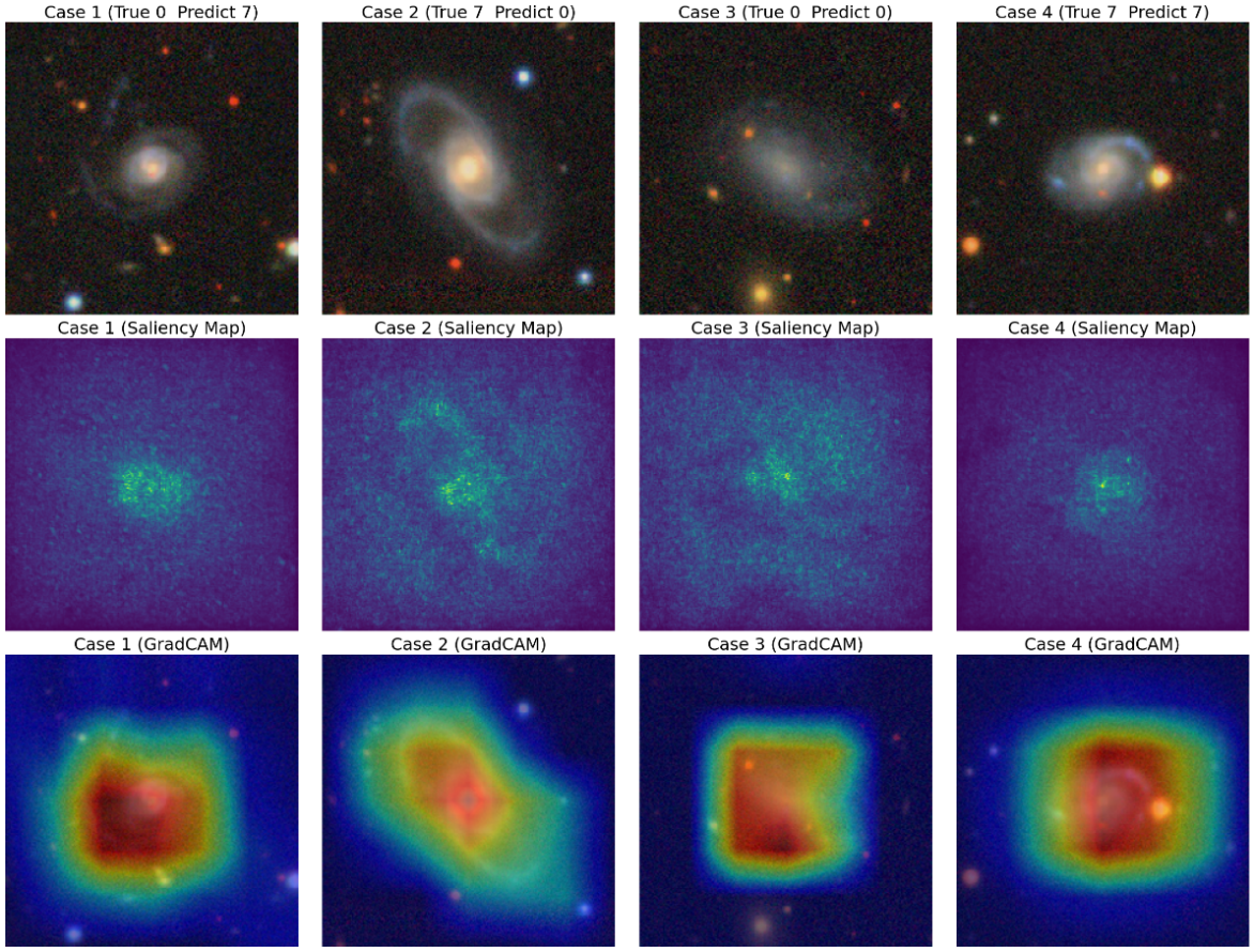
Figure 8. Salience maps and Grad-CAM for 4 cases predicted by the DenseNet-T1 (dropout rate 0.3).

3.2. Model comparison

Figure 9 and 10 exhibit boxplots showcasing the best validation accuracy and training accuracy of models for each architecture. The green boxes represent the interquartile range of the accuracy for each architecture. The blue triangle makers represent the average values of the accuracy for each architecture, and the red lines represent the medium values. However, the outliers are not shown in the figure. As shown in Figure 9 and Figure 10, the performance of models that utilize the EfficientNetB0 as pre-trained model are much more consistent than the ones that utilize the DenseNet121. Especially with training accuracy, when the designs of fully connected layers are the same, models using the EfficientNetB0 have higher medium and maximum values of accuracy. However, models using the DenseNet121 and global average pooling outperform other models significantly on validation set, with accuracy 1% to 2% higher than others. This may be because the DenseNet121 has much more convolutional layers than the EfficientNetB0, thus it can extract features with higher complexity. Meanwhile, the EfficientNetB0 may only learn edges and shapes, which can be very similar between some classes, leading to more misclassification on validation set.

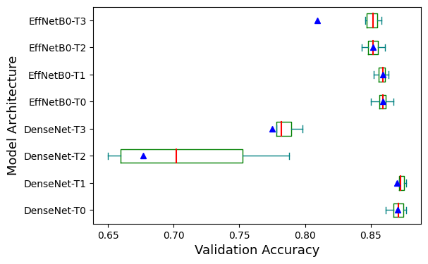Figure 9. Validation accuracy of models for each architecture.

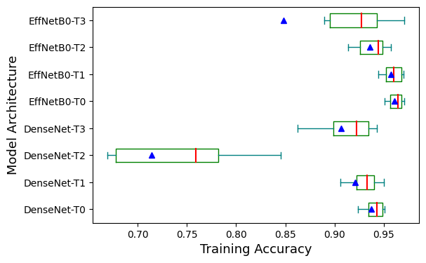Figure 10. Training accuracy of models for each architecture.

Figure 11 and Figure 12 respectively illustrate how different dropout rates affect the overall performance of models using DenseNet121 and models using EfficientNetB0. Comparing these two figures, the plots for average validation accuracy fluctuate when the dropout rate is between 0% and 70%. A sharp drop can be observed in both figures once the dropout rate is increased to 80%. This means that in general, an excessive dropout rate in fully connected layers damages the overall performance of CNNs, while regular dropout rates cannot efficiently improve model performance despite the architecture of the fully connected layers. However, as shown in Figure 12, when the dropout rate is between 10% and 70%, the interquartile ranges of accuracy are much narrower than the one without dropout. This indicates that for CNNs with lower complexity, dropout in fully connected layers can improve consistence and reduce the impact of the design of fully connected layers on the overall performance. This may be due to the fact that CNNs with less convolutional layers may learn more irrelevant representation and shallow features for classification. Dropout in the fully connected layers can force the networks to learn more from extracted features, and automatically function as feature selection during the training process, which improves feature utilization and relevance for more stable results.

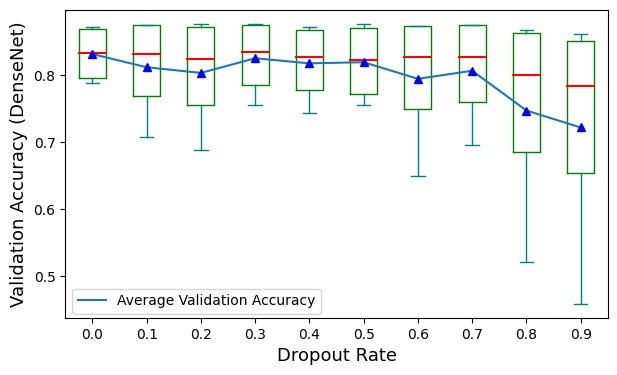
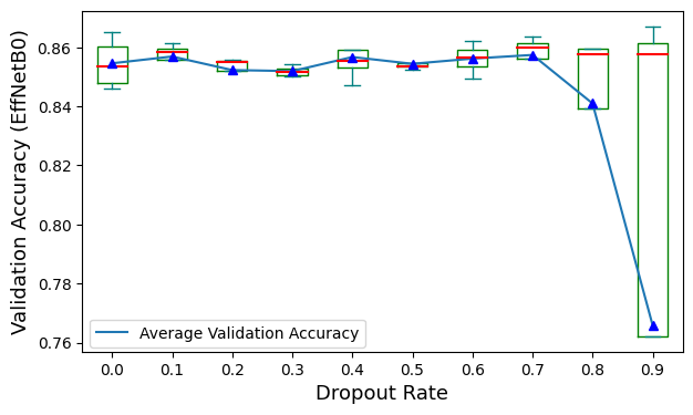
Figure 11. Validation accuracy of models using DenseNet121 for each dropout rate.

Figure 12. Validation accuracy of models using EfficientNetB0 for each dropout rate.

Figure 13 illustrates how different dropout rates affect the overall performance of models with different architectures for fully connected layers. As shown in Figure 13, models using architecture T0 and T1 obtained much better accuracy than others. This is because Global Average Pooling can represent features better than flattening, and it can reduce model complexity efficiently. Although different dropout rates do not seem to improve model performance for architecture T0, T2 and T3, however, an increase can be observed for architecture T1 when the dropout rate is between 20% and 50%, and the maximum value appears at 40%. This indicate that dropout can be used in fully connected layers with GAP and complex design. It may improve performance and avoid overfitting.

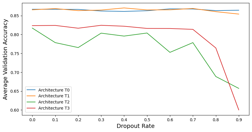
Figure 13. Average validation accuracy of models with different architectures for fully connected layers versus dropout rates.

4. Conclusion

This paper compared the performance of different models for galaxy classification and investigated how different dropout rates impact the overall performance of the DenseNet121 and EfficentNetB0 with four types of fully connected layers. Techniques including transfer learning, data argumentation, and learning rate decay are utilized to improve the overall performance of CNNs. Saliency maps and grad-CAM are used for model interpretation. Experimental results from model comparison show that the effect of dropout rates on the overall performance is insignificant comparing to the effect of architectures, but an excessive dropout rate in fully connected layers can reduce model performance substantially. However, results also indicate that for CNNs with relatively low complexity, the utilization of dropout with a proper rate in fully connected layers can increase model consistency and robustness, leading to better performance with less parameters. For future works, different learning rate schedules should be investigated based on different CNNs, and various CNNs with less parameters should be tested to compare the effect of dropout rate on model performance.

References

[1]. Lauer T R et al 2021 New Horizons observations of the cosmic optical background The Astrophysical Journal 906.2 77
[2]. Hubble E 1934 The distribution of extra-galactic nebulae The Astrophysical Journal 79 8
[3]. Schawinski K et al 2007 Observational evidence for AGN feedback in early-type galaxies Monthly Notices of the Royal Astronomical Society 382.4 pp 1415-1431
[4]. Dieleman S et al 2015 Rotation-invariant convolutional neural networks for galaxy morphology prediction Monthly notices of the royal astronomical society 450.2 pp 1441-1459
[5]. Aniyan A K et al 2017 Classifying radio galaxies with the convolutional neural network The Astrophysical Journal Supplement Series 230.2 20
[6]. Zhu X P et al 2019 Galaxy morphology classification with deep convolutional neural networks." Astrophysics and Space Science 364 pp 1-15
[7]. Becker B et al 2021 CNN architecture comparison for radio galaxy classification." Monthly Notices of the Royal Astronomical Society 503.2 pp 1828-1846
[8]. Hui W Y et al 2022 Galaxy Morphology Classification with DenseNet Journal of Physics: Conference Series vol 2402 no 1 IOP Publishing
[9]. Dileep P et al 2020 Dense layer dropout based CNN architecture for automatic modulation classification 2020 national conference on communications (NCC) IEEE
[10]. Walmsley M et al 2022 Galaxy Zoo DECaLS: Detailed visual morphology measurements from volunteers and deep learning for 314 000 galaxies Monthly Notices of the Royal Astronomical Society 509.3 pp 3966-3988
[11]. Haralick R M et al 1987 Image analysis using mathematical morphology IEEE transactions on pattern analysis and machine intelligence 4 pp 532-550
[12]. LeCun Y et al 1998 Gradient-based learning applied to document recognition Proceedings of the IEEE 86.11 pp 2278-2324
[13]. Arena P Basile A Bucolo M et al 2003 Image processing for medical diagnosis using CNN Nuclear Instruments and Methods in Physics Research Section A: Accelerators, Spectrometers, Detectors and Associated Equipment 497(1) pp 174-178
[14]. Yu Q Wang J Jin Z et al 2022 Pose-guided matching based on deep learning for assessing quality of action on rehabilitation training Biomedical Signal Processing and Control 72: 103323
[15]. Sun Y Xue B Zhang M et al 2018 Automatically evolving cnn architectures based on blocks arXiv preprint arXiv:1810.11875
[16]. Huang G et al 2017 Densely connected convolutional networks Proceedings of the IEEE conference on computer vision and pattern recognition pp 4700-4708
[17]. Tan M X et al 2018 Efficientnet: Rethinking model scaling for convolutional neural networks International conference on machine learning PMLR pp 6105-6114
[18]. Tan M X 2018 MnasNet: Towards Automating the Design of Mobile Machine Learning Models arXiv:1807.11626
Cite this article
Hu,H. (2023). Galaxy classification based on convolutional neural networks with dropout technique. Applied and Computational Engineering,22,42-52.
Data availability
The datasets used and/or analyzed during the current study will be available from the authors upon reasonable request.
Disclaimer/Publisher's Note
The statements, opinions and data contained in all publications are solely those of the individual author(s) and contributor(s) and not of EWA Publishing and/or the editor(s). EWA Publishing and/or the editor(s) disclaim responsibility for any injury to people or property resulting from any ideas, methods, instructions or products referred to in the content.
About volume
Volume title: Proceedings of the 5th International Conference on Computing and Data Science
© 2024 by the author(s). Licensee EWA Publishing, Oxford, UK. This article is an open access article distributed under the terms and
conditions of the Creative Commons Attribution (CC BY) license. Authors who
publish this series agree to the following terms:
1. Authors retain copyright and grant the series right of first publication with the work simultaneously licensed under a Creative Commons
Attribution License that allows others to share the work with an acknowledgment of the work's authorship and initial publication in this
series.
2. Authors are able to enter into separate, additional contractual arrangements for the non-exclusive distribution of the series's published
version of the work (e.g., post it to an institutional repository or publish it in a book), with an acknowledgment of its initial
publication in this series.
3. Authors are permitted and encouraged to post their work online (e.g., in institutional repositories or on their website) prior to and
during the submission process, as it can lead to productive exchanges, as well as earlier and greater citation of published work (See
Open access policy for details).