1. Introduction

In modern society, national income is an important economic indicator that reflects the overall level of a country or region's economy and the quality of life of its people. The prediction and analysis of national income is of great significance to governments, policy makers and individuals, and can provide powerful decision support for economic policy making, resource allocation and personal financial planning. With the rapid development of machine learning and data science, machine learning algorithms such as logistic regression and decision trees are widely used in the field of economics, providing economists and researchers with new tools and methods to forecast and analyze national income. Logistic regression is a supervised learning algorithm for classification problems, while decision trees are algorithms that can extract decision rules from data [1]. By combining logistic regression and decision trees prediction models can be built to make accurate predictions of whether national income is above a specific threshold.

The main objective of this study is to explore the relationship between national income and other related factors using logistic regression and decision tree models, and to build prediction models to achieve accurate predictions of national income. By collecting and analyzing a large amount of economic data, this paper will investigate the association between national income and factors such as demographic characteristics, education level, and industry structure, and use machine learning algorithms for model training and prediction.

Prediction of whether national income is above a certain threshold through logistic regression and decision trees can provide valuable information and decision support for individuals, households, governments, and policy makers, while also promoting the intersection of economics and machine learning at the application level. These studies have important implications and value for economic decision making, resource allocation and economic development of individuals and societies.

2. Data

2.1. Data resource

This project will use data collected by the U.S. Census and select supervised learning algorithms to accurately model and predict the income of respondents. The goal of this paper is to develop a model that can accurately predict whether a respondent's annual income exceeds $50,000 [2]. The data used in this paper were obtained from Kohavi and Becker.

2.2. Basic Data Information

2.2.1. Missing values

To ensure the metrics of the data, the dataset was viewed for missing values. There are no missing values for each feature of the data and the numerical quality is excellent. Descriptive statistics were calculated for the numerical features and the mean, variance, and median information of each column feature were viewed as shown in Table 1. It is found that the distribution interval of capital-gain and capital-loss columns is relatively large, which is a trailing situation, and logging is performed to make their distribution more normal.

Table 1. Data descriptive statistics

2.2.2. Distribution of the characteristics of each category

As shown in Table 2, the distribution of each category feature is relatively normal. However, since the category features cannot be brought into the model for calculation, they are transformed by the unique thermal coding process.

Table 2. Part of the category characteristics distribution

2.3. Data Analysis

2.3.1. Numerical characterization. Age and hours worked per week are chosen for this analysis, and the age characteristics are divided into national income categories (over $50,000 or not) and then visualized in a box plot. For the number of hours worked per week, the mean value of the number of hours worked per week for different income categories is calculated and then plotted as a bar chart, as shown in Figure 1. In terms of age distribution, the age of those earning >$50,000 is generally higher than that of those earning <$50,000, indicating that the older the person is, the more likely he or she is to earn more than $50,000. In terms of the average number of hours worked per week, those earning >$50,000 also work more hours per week than those earning <$50,000. The average number of hours worked per week for those earning >$50,000 is 45.5 hours, compared to 38.8 hours for those earning <$50,000, which shows that hours worked are an important factor in income.

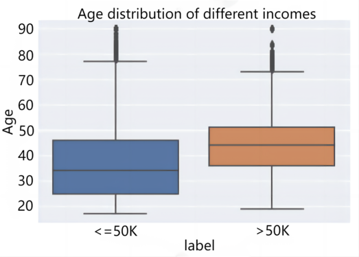
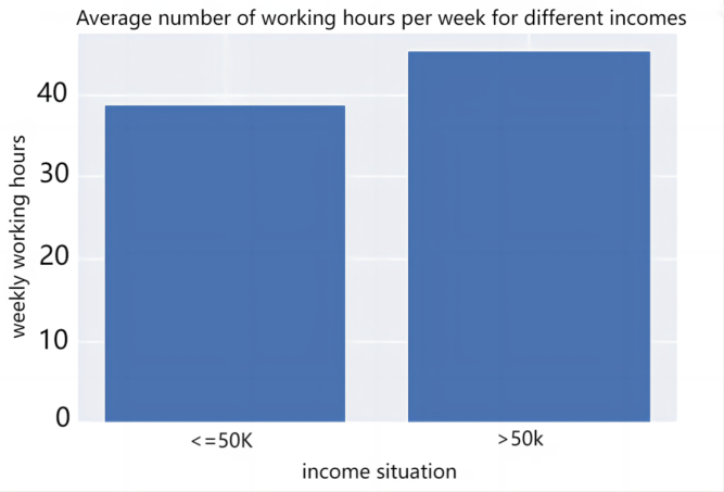
Figure 1. Average weekly hours worked by income category: (a)Age distribution of different incomes, (b)Average number of working hours per week for different incomes.

2.3.2. Category type feature analysis. For the analysis of category-based characteristics, the analysis is performed by calculating the proportion of >$50,000 versus <=$50,000 for different types of fetching values separately and presenting it with a stacked bar chart. Importantly, the proportions of income groups under different job types, marital status, family roles, and gender were analyzed, and the results are shown in Figure 2.

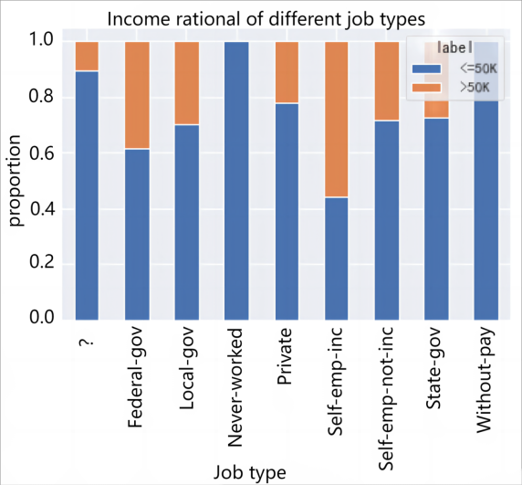
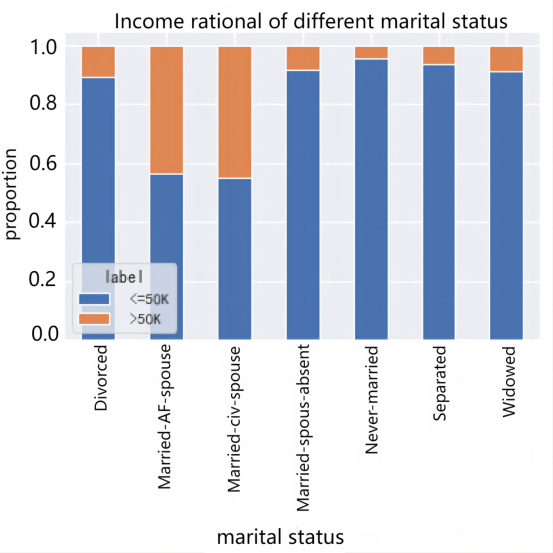
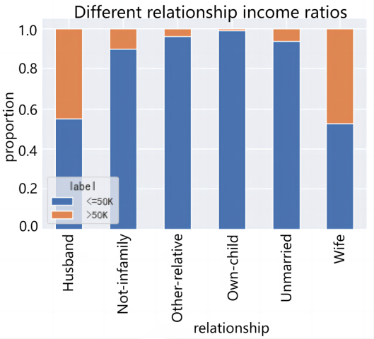
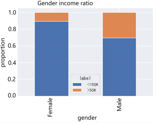
Figure 2. Category type feature analysis: (a)Income ratio of different job types, (b)Income ratio of different marital status, (c)Different relationship income ratios, (d)Gender income ratio.

From Figure 2, the effect of different types of earnings on income is also obvious. Without-pay and Never-worked are both below $50,000 because of the small base. From the perspective of marital status, Married-AF-spouse and Married-civ-spouse have the highest percentage of high-income people reaching about 50%, while Married-spouse-absent is the lowest at less than 1%. In terms of family roles, Husband and Wife high income ratio is the highest, both above 40%, which indicates that stable family income will also be a little higher. But Own-child's high income proportion is the lowest less than 1%. In terms of gender, Male's income is higher, with 30.1% of the high income group, which is larger than Female's high income group (10.9%).

2.4. Feature processing of data

2.4.1. Basic processing. The label Label is processed, and <=50K and >50K are converted to 0-1 using {' <=50K':0,' >50K':1} rules to facilitate the subsequent construction of the classification model. Since the features education and education-num are duplicated, the education feature is removed. Since the distribution intervals of the capital-gain and capital-loss features were found to be relatively large, the log(x+1) display was used to convert them to a certain degree for the tilt correction.

2.4.2. Normalization process. In order to prevent the problems caused by the different scales of the data, the numerical data are normalized to remove the effects of scale. A linear transformation is performed on the original data using min-max normalization, so that the results are mapped to the range [0,1] and the data are of the same size. The numerical characteristics 'age', 'education-num', 'capital-gain', 'capital-loss', and 'hours-per-week' were processed, and some of the processed data are shown in Table 3.

Table 3. Normalization results

2.5. Unique heat code

Since there are many category features in the data that cannot be brought into the subsequent model for computation, they need to be processed using unique thermal coding. Because the sizes of the attributes of the unordered features cannot be compared among themselves, it is usually required that the unordered features (called unordered category variables) be transformed. A popular approach to unordered transformed category variables is to use a unique heat encoding scheme. The unique heat encoding creates a "dummy" variable for each possible category of each unordered categorical feature [3]. For example, suppose someFeature has three possible values A, B, or C. This feature is encoded as someFeature_A, someFeature_B, and someFeature_C. Some of the results for each particular feature after the unique heat encoding process are shown in Table 4:

Table 4. Unique heat code processing results

3. Logistic regression

The logistic regression algorithm is often applied in dichotomous problems, where the data with N-dimensional characteristics in dichotomous problems, each independent variable x corresponding to y takes only two possible values 0 or 1. Due to the characteristics of the logistic regression model, it has a relatively good performance in solving dichotomous models. Logistic regression is a multivariate analysis method that studies the relationship between the dependent variable as a dichotomous or multicategorical observation and the influencing factor (independent variable) and is a probabilistic nonlinear regression [4]. Logistic regression predicts the classification of a sample by creating a logistic function (also called Sigmoid function).

3.1. Fundamentals

The basic principle of logistic regression is by mapping the output values of a linear regression model into a probability interval and then classifying them according to a threshold. Its output in the prediction problem is a probability value that represents the probability that the sample belongs to a certain category. Logistic regression assumes that the output variables of the sample obey the Bernoulli distribution, i.e., the binomial distribution. The output of the linear regression model is restricted to between 0 and 1 by applying a logistic transformation to it, indicating the probability that the sample belongs to a certain category [5]. The logistic function used in logistic regression is the Sigmoid function, which has an S-shaped curve that maps the real numbers between 0 and 1. The logistic regression model representation is shown below.

\( {h^{θ}}(x)=g({θ^{T}}*x) \)

where

\( {h^{θ}}(x) \) denotes the probability that the sample \( x \) belongs to the positive class,,

\( g(z) \) denotes the logistic function (Sigmod function),

\( θ \) is the parameter vector of the model,

\( x \) is the feature vector of the output sample.

The model training process of logistic regression usually uses maximum likelihood estimation or gradient descent method. Maximum likelihood estimation is a commonly used parameter estimation method to select the optimal parameters by maximizing the likelihood function. Gradient descent is an optimization algorithm that minimizes the loss function by iteratively updating the parameters. The key to training a logistic regression model is to define the loss function and choose a suitable optimization algorithm. A commonly used loss function is the log loss function (log loss), which is used to measure the difference between the predicted probability and the true label. Commonly used optimization algorithms include gradient descent, stochastic gradient descent, and Newton's method.

3.2. Experimental

Logistic regression does not have a particularly large number of hyperparameters to be adjusted, so the LogisticRegression() model in sklearn is used for logistic regression model building. The training set is used to model the parameters of the logistic regression model, and then the test set is used to see how well the model predicts the unknown data set. After obtaining the model, the model was used to predict the training set and the test set and to calculate each classification index to observe the performance of the model (Table 5):

Table 5. Results of logistic regression indicators

The prediction results of the logistic regression model on the training and test sets are plotted as ROC curves as shown in Figure 3. From Figure 3, the logistic regression model performs well in terms of accuracy, reaching 0.7+ in both the training and test sets, but the AUC performance is poor at about 0.5.

Therefore, from the two classification results, logistic regression cannot predict the national income with comparable accuracy.

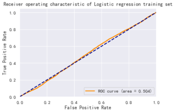
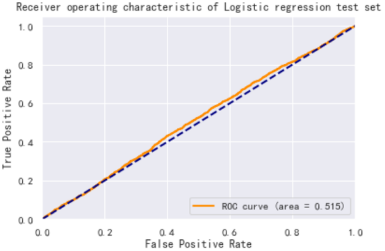
Figure 3. The prediction results of the logistic regression model: (a) Receiver operating characteristic of Logistic regression training set, (b)Receiver operating characteristic of Logistic regression test set

4. Decision tree

The decision tree algorithm is an inductive instance-based learning method that inductively obtains a tree model from some unordered data. Each intermediate node of the tree model records which threshold value based on which feature is used to classify the data, and the leaf nodes in the tree model represent the final judged category [6]. When a new data comes over to judge the classification, the data is divided and categorized by the tree path obtained from the training.

4.1. Principles

The basic principle of the decision tree algorithm is to generate a tree structure by recursively partitioning the dataset such that each internal node represents an attribute test and each leaf node represents a category label or regression value. Based on the different types of attributes, decision tree algorithms can be divided into two types: classification trees and regression trees [7].

4.1.1. Classification trees. Classification trees are used to handle the classification task, which divides the data set into different categories. In classification trees, each leaf node represents a category label and each internal node is tested based on the attribute values and divides the dataset into different sub-nodes until a predefined stopping condition is reached (e.g., purity reaches a certain threshold or maximum depth is reached).

4.1.2. Regression tree. The regression tree is used to handle the regression task, which divides the dataset into different intervals of values. In a regression tree, each leaf node represents a numerical output and each internal node is tested based on attribute values and divides the data set into different sub-nodes until a predefined stopping condition is reached.

4.2. Theoretical basis

The decision tree algorithm is a supervised learning algorithm based on a tree structure for solving classification and regression problems. Its theoretical basis includes the following aspects [8]:

4.2.1. Information theory and entropy. The basic idea of decision tree algorithm is to divide the data set by selecting the optimal features according to the concept of information theory, so that each divided subset has less purity or uncertainty in the target variable. Entropy is a measure of uncertainty used in information theory, and a common measure used in decision tree algorithms is the information gain (or information gain rate), which is the difference between the entropy of the original set and the entropy of the partitioned subsets.

4.2.2. Recursive partitioning and greedy strategy. The decision tree algorithm uses recursive partitioning to construct a decision tree, i.e., by selecting the best features to partition the dataset and further partitioning each partitioned subset recursively as a new dataset until the stopping condition is satisfied. At each division, the decision tree algorithm uses a greedy strategy to select the current best feature for the division in the expectation of better overall results.

4.2.3. Feature selection and partitioning criteria. The decision tree algorithm divides by selecting the best features to make the divided subset more pure. Commonly used feature selection criteria include information gain, information gain rate, Gini index, etc. These criteria evaluate the importance of the features during the computation and select the features with better classification ability for division.

4.2.4. Pruning Strategy and Model Complexity. Decision tree algorithms are prone to overfitting problems, i.e., they perform well on training data but have poor generalization ability on new data. To solve the overfitting problem, the decision tree algorithm introduces a pruning strategy, i.e., after constructing a complete decision tree, some nodes or subtrees are pruned to reduce the model complexity and improve the generalization ability.

4.3. Construction process

The process of constructing a decision tree algorithm can be divided into the following steps:

4.3.1. Feature selection. The best attribute is selected as the division attribute of the current node. Commonly used feature selection criteria include information gain, information gain ratio, Gini index, etc [9].

4.3.2. Node partitioning. According to the selected division attributes, the dataset is divided into multiple sub-datasets, and each sub-dataset corresponds to a child node.

4.3.3. Recursive construction. For each sub-node, steps 1 and 2 are repeated until a predefined stopping condition is reached (e.g., purity reaches a certain threshold or maximum depth is reached), or the dataset is empty.

4.3.4. Leaf node labeling. Assign a category label or regression value to each leaf node, which is usually determined using majority voting or the mean.

4.4. Experimental

This paper use the DecisionTreeClassifier () model in sklearn for decision tree model building. First, we use the training set to model the parameters of the decision tree model, and then we use the validation set to see how the model performs for unknown data. Since the decision tree has more hyperparameters, it needs to be adjusted, and the main parameters are max_depth and min_samples_split. As a result, the model works better when the parameters are max_depth = 9 and min_samples_split = 4 after several tests.

The performance of the decision tree model in the training and validation sets for ACC and AUC metrics is further calculated as shown in Table 6:

Table 6. Decision tree indicator results

And the prediction results of the decision tree model on the training and test sets are plotted as ROC curves as shown in Figure 4. Based on Figure 4, the prediction results of the decision tree model are very good, with the ACC indicator results of 0.86+ on both the training and test sets, and the AUC results of 0.9+. This indicates that the model can accurately predict whether the national income is greater than $50,000.

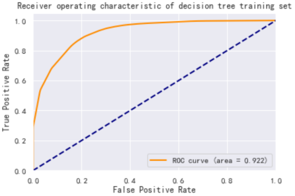
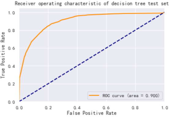
Figure 4. The prediction results of the decision tree model: (a)Receiver operating characteristic of decision tree training set, (b)Receiver operating characteristic of decision tree test set

5. Limitation

5.1. Limitations and challenges of logistic regression:

Logistic regression is based on the assumption of linearity, assuming a linear relationship between characteristics and national income. However, in real situations, national income is affected by multiple factors and may have nonlinear relationships, so logistic regression models may not capture the complex relationships well. Logistic regression models usually cannot directly deal with nonlinear relationships and interactions between features. The predictive performance of logistic regression models may be limited if there are nonlinear relationships or interactions between features. In addition, logistic regression models are sensitive to outliers, i.e., a few outliers may have a large impact on the parameter estimation and prediction results of the model. This may lead to a decrease in the stability and robustness of the model. Logistic regression models are relatively difficult to handle missing values and usually require the conversion of categorical features to numerical features. This involves the processing of feature engineering and may lead to loss of information or introduction of bias.

5.2. Limitations and Challenges of Decision Trees:

Decision trees are prone to overfitting, especially when the depth of the tree is large or the training samples are small. Overfitting can lead to models that perform well on training data but generalize poorly on new data. Decision trees are very sensitive to small changes in the input data, i.e., minor data changes may result in a completely different tree structure [10]. This makes decision trees less stable in some cases and more sensitive to data noise and outliers. Decision trees are usually used to handle continuous features by thresholding the divisions. However, it is a challenge to choose the appropriate division point and division strategy for the processing of continuous features. Different division methods may lead to different decision tree structures and prediction results. Decision trees face challenges when dealing with high-dimensional data. As the number of features increases, the complexity and computational complexity of decision trees also increase, which can easily lead to dimensional disasters and overfitting problems.

6. Conclusion

In this paper, we mainly used python's numpy and pandas to clean and pre-process the data, normalize, and unique hot coding, and then completed the visual analysis exploration of the factors affecting income, including the type of work, marital status, and family roles, etc. using matplotlib and seaborn. The analysis shows that men have a higher proportion of high income than women, and the older the group, the higher the income is likely to be, and the higher the number of hours worked per week is likely to be. Two models, logistic regression and decision tree, are used to calculate ACC and AUC indicators respectively using sklearn library, and the models are judged to be good or bad. Through the comparison of operations and results, the decision tree is proved to be the current optimal prediction model. However, both logistic regression and decision tree based algorithms have some problems when forecasting national income. Therefore, other machine learning algorithms or suitable feature engineering, data preprocessing and model tuning methods can be considered to improve the forecasting performance.

References

[1]. Y. K. Liu. A disk failure prediction system based on machine learning [D]. Huazhong University of Science and Technology,2015.
[2]. Tan Bo,Pan Qingwen,Cheng Wen. GBDT-based individual income level prediction[J]. Computer and Digital Engineering,2020,48(03):550-552+602.
[3]. Liang J, Chen JH, Zhang Xueqin et al. Anomaly detection based on unique thermal coding and convolutional neural network[J]. Journal of Tsinghua University (Natural Science Edition),2019,59(07): 523-529.DOI:10.16511/j.cnki.qhdxxb.2018.25.061.
[4]. Chen J,Liu Zunxiong. Spam filtering based on non-negative matrix decomposition feature extraction[J]. Journal of East China Jiaotong University,2010,27(06):75-79.
[5]. Li Zhuo Ran. Principles and applications of logistic regression methods[J]. China Strategic Emerging Industries, 2017(28): 114-115.DOI:10.19474/j.cnki.10-1156/f.001686.
[6]. Chen J. Credit bond default risk measure based on KMV-random forest model [D]. Shanghai University of Finance and Economics, 2020. DOI:10.27296/d.cnki.gshcu.2020.000571.
[7]. Wang Jingxiang. Principle research and practical application of decision tree algorithm[J]. Computer Programming Skills and Maintenance, 2022, No.446(08): 54-56+72.DOI:10.16184/j.cnki.comprg.2022.08.043.
[8]. Belen Wang. Machine learning [M]. Nanjing Southeast University Press:, 202111.355.
[9]. Feng, X. H.. Research on fuzzy decision tree algorithm based on axiomatic fuzzy sets [D]. Dalian University of Technology, 2013.
[10]. Xue-Chen Zhang,Yuan-Yuan Zheng,Yao Chen. Research on early warning technology of thunderstorm and windy weather based on decision tree method[C]//Chinese Meteorological Society.S1 Disaster Weather Research and Forecasting. [publisher unknown],2012:5.
Cite this article
Sun,W. (2023). Research on the national income prediction based on Python. Applied and Computational Engineering,22,53-62.
Data availability
The datasets used and/or analyzed during the current study will be available from the authors upon reasonable request.
Disclaimer/Publisher's Note
The statements, opinions and data contained in all publications are solely those of the individual author(s) and contributor(s) and not of EWA Publishing and/or the editor(s). EWA Publishing and/or the editor(s) disclaim responsibility for any injury to people or property resulting from any ideas, methods, instructions or products referred to in the content.
About volume
Volume title: Proceedings of the 5th International Conference on Computing and Data Science
© 2024 by the author(s). Licensee EWA Publishing, Oxford, UK. This article is an open access article distributed under the terms and
conditions of the Creative Commons Attribution (CC BY) license. Authors who
publish this series agree to the following terms:
1. Authors retain copyright and grant the series right of first publication with the work simultaneously licensed under a Creative Commons
Attribution License that allows others to share the work with an acknowledgment of the work's authorship and initial publication in this
series.
2. Authors are able to enter into separate, additional contractual arrangements for the non-exclusive distribution of the series's published
version of the work (e.g., post it to an institutional repository or publish it in a book), with an acknowledgment of its initial
publication in this series.
3. Authors are permitted and encouraged to post their work online (e.g., in institutional repositories or on their website) prior to and
during the submission process, as it can lead to productive exchanges, as well as earlier and greater citation of published work (See
Open access policy for details).