1. Introduction

The year 2022 is a significant year for the global options market, marking the first instance of new options being listed since 2019, encompassing a variety of options types such as stock index and Full name ETF options, and across several trading venues, including the China Financial Exchange, Shanghai Stock Exchange, and NASDAQ Stock Exchange. From the perspective of historical performance, the listing of new option varieties is expected to significantly stimulate the current option trading heat. In the case of the overall weakness of the stock market in 2022, the total growth rate of the option position remained above 20%. Since the listing of the new option, the daily average position has risen steadily and maintained a high growth momentum. The factors that affect the basis of equity futures can be divided according to the length of the period: long-term stable long and short position game, short-term market sentiment and put option hedging position adjustment, and cyclical dividend effect. It is believed that the convergence of the basis at the end of 2023 may be attributed to several factors. In the short term, the effect of stabilizing the real estate and opening up the policy gradually appears, and the stock index futures should be more optimistic about the trend of the index in the coming months. In addition, when the index falls, the hedging position of put option products also makes the price of stock index futures rise instead of falling compared with the spot price because of its hedging characteristics of "high selling and low absorbing".

In conjunction with foreign research findings, the present study employs Convolutional Neural Networks to construct a range of sub-indicators that capture the liquidity and volatility of financial assets, subsequently utilizing these sub-indicators to develop comprehensive measures of liquidity and volatility. To price volatility for multiple assets, the lognormal random walk theory is applied to each asset dimension, and the value of European options independent of path is obtained via multiple integration. The essence of the pricing of such options is to calculate the integral, which will become very inefficient in the case of high dimension and orthogonality, and Monte Carlo method can solve this problem [1]. The principle of Monte Carlo integral estimation is simple: integral is the average value multiplied by a quantity, which is a continuous accumulation process. The average value can be estimated by random number, with time complexity of O (N) and accuracy of O (1/N1/2), which is independent of dimension [2]. In the 1960s, scholars have carried out a lot of research on low-deviation sequences, and proved that non-random distribution can reach the accuracy of O (1/N) (there may be small correlation between dimensions). Nowadays, once random numbers are needed, low-deviation sequences are still a very useful tool, and are also widely used in the field of option pricing [3]. In the early 1990s, many scholars (Cheyette, Barrett, Moore, Wilmott, etc.) expanded upon their previous achievements and delved deeper into the problem of the multi-asset option pricing. They applied the knowledge of number theory to the financial field in terms of volatility, each index has obvious amplification of volatility, but the direction and amplitude of fluctuation among the indexes are relatively consistent, without obvious difference [4]. There is no obvious change in the time distribution of the transaction. In the long run, it may also be the recent slowdown in the growth of neutral strategy products [5]. Another possible reason is that the continuous listing of option products in the second half of the year has increased the richness of hedging tools, dispersed the demand for long hedging and reduced the overall strength of short positions in stock index futures. These developments have given rise to the need for effective multi-party data and increased the demand for efficient Artificial Intelligence (AI) models [6].

Combining the micro-characteristics of each index and the performance of high-frequency trading in data, deep learning will play a greater role. This study will involves leveraging LGB and other models to efficiently exploit data to create high returns, achieve the highest sharp ratio, and use the effective stock market factor to re-open the return window in the current environment of epidemic recovery and global recession.

2. Method

2.1. Dataset description

The present dataset has been sourced from a reputable global market maker and can be accessed through Kaggle. This dataset, which describes Optiver Realized Volatility Prediction, includes order book snapshots and executed trade data that are important for trade execution in the financial markets. In particular, some variables used for the main research are fully and truly supported, such as the returns that are widely used in the financial industry, but whenever some mathematical models are needed, it is better to use logarithmic returns.

The standard deviation of stocks' logarithmic returns serves as an important input to our model when we trade options. Since the standard deviation of the logarithmic return will fluctuate depending on whether it is calculated over a longer or shorter time period, it is typically normalized to a one-year period. This annualized standard deviation is known as volatility.

The order book is also one of the main sources of stock valuation. The valuation based on fair book value must consider two factors: the level and size of the order. In this competition, we use the Weighted Average Price (WAP) to calculate the instantaneous valuation of stocks and take the realized volatility as our goal. Figure 1 and Figure 2 present the weighted average price and logarithmic returns, respectively.

\( σ=\sqrt[]{\sum _{t}r_{t-1,t}^{2}} \) (1)

\( WAP=\frac{{BidPrice_{1}}*{AskSize_{1}}+{AskPrice_{1}}*{BidSize_{1}}}{{BidSize_{1}}+{AskSize_{1}}} \) (2)

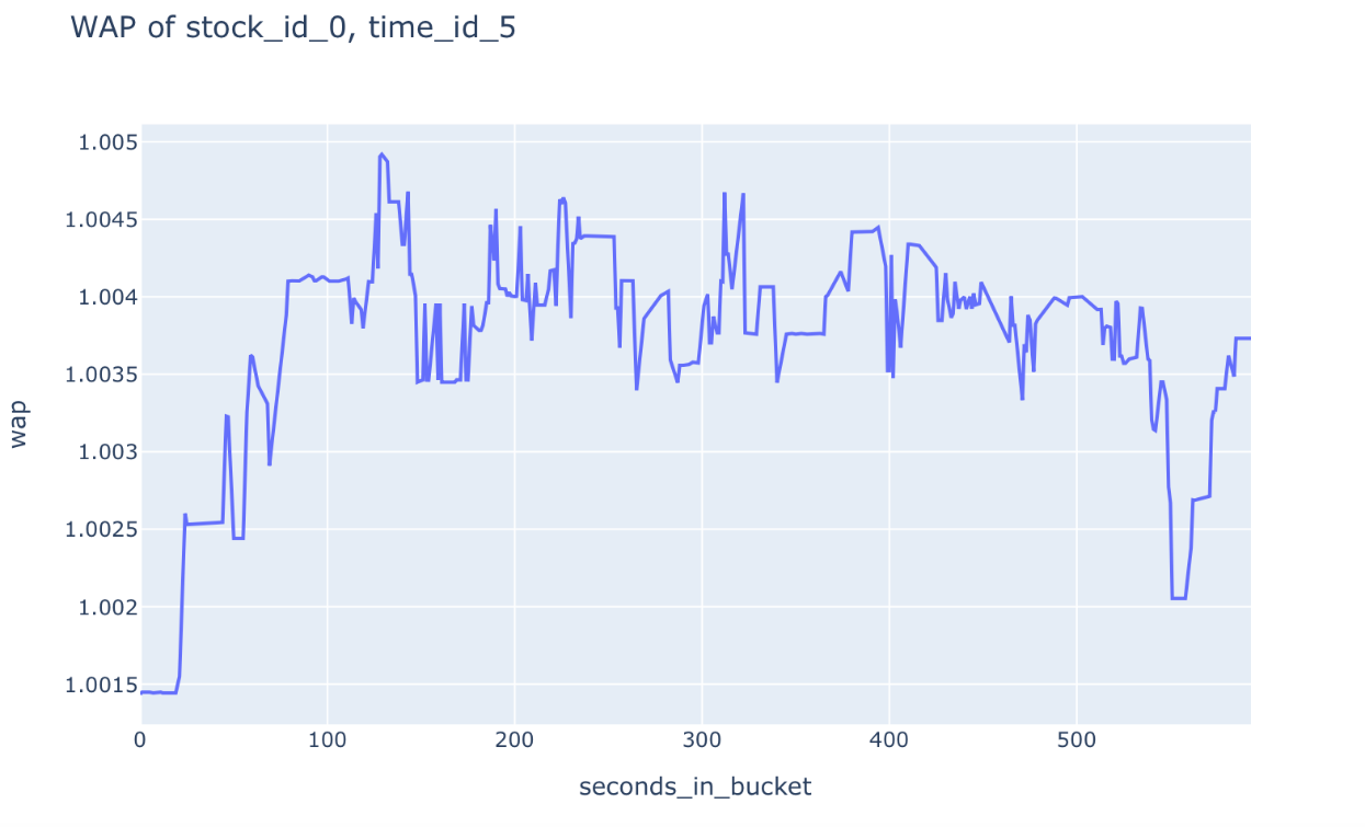
Figure 1. Weighted average price.

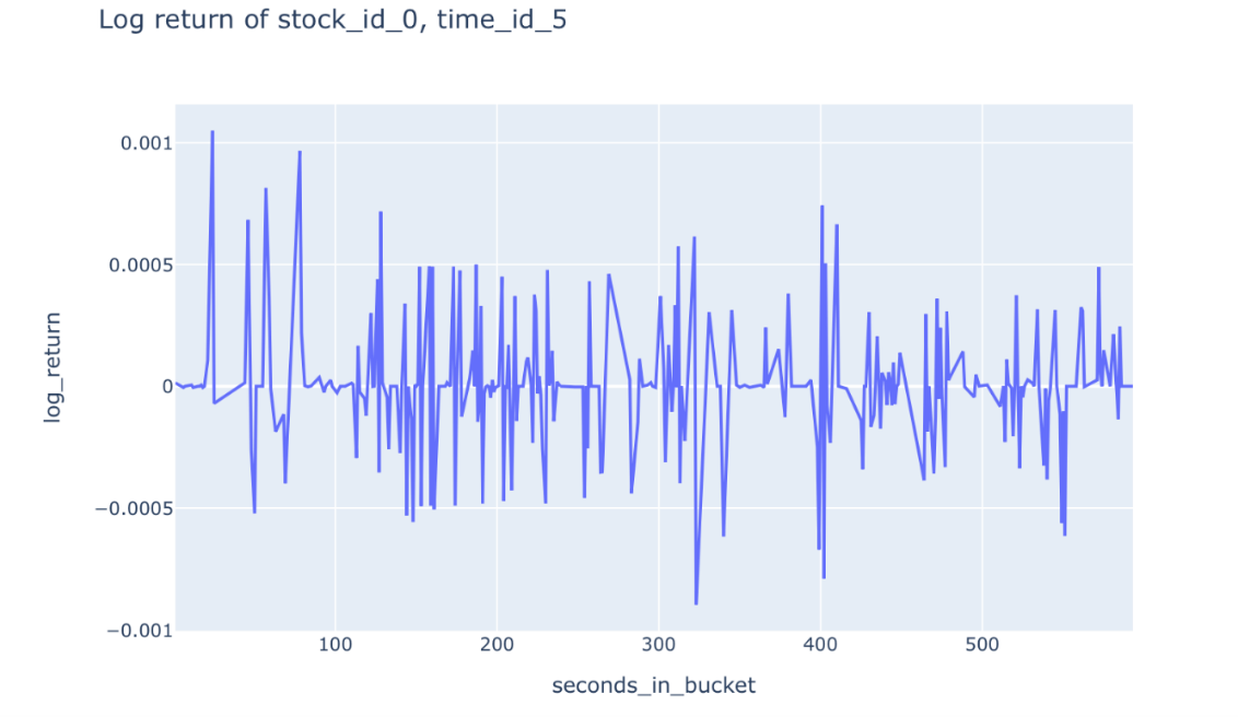
Figure 2. logarithmic returns.

It permits fine-grained studies of the microstructure of contemporary financial markets at a resolution of one second. The test set utilized includes information that can be used to create features and can foretell information for around 150,000 target values. According to our estimates, loading the entire dataset may consume more than 3 GB of memory. During the training phase of the competition, most of the test data will be populated to ensure that the dataset size is essentially the same as the actual test data. However, during the real forecasting phase, the filler data will be substituted with market data.

2.2. Machine learning models

Machine learning models such as Light Gradient Boosting Machine (LGBM) and Recurrent Neural Networks (RNN) have shown great promise in the field of finance, particularly in the stock and options markets.

2.2.1. Light Gradient Boosting Machine. LGBM, in particular, has gained popularity due to its high efficiency, scalability, and accuracy compared to other boosting models. One of the major advantages of LGBM is its ability to handle large datasets with high dimensional features. The algorithm employs a leaf-wise approach, which selects the leaf node that will result in the maximum decrease in the loss function. This technique enables LGBM to construct deeper and narrower decision trees, leading to a more efficient and accurate model. Moreover, LGBM supports parallel computing, enabling it to process large datasets much faster such as financial time series data, and can efficiently extract features and patterns from large datasets [7]. LGBM has been used to predict stock prices, identify potential trading opportunities, and optimize portfolio management strategies. And LGBM model utilizes the special structure of Leaf-wise growth strategy, left_childs assigns 5 internal points (1,3,-2,-1,4), the right_childs gives 5 points to structure.(2,-3,4,-5,6).

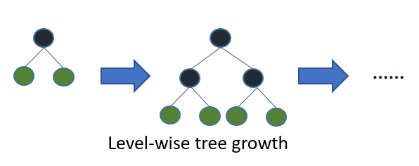
Figure 3. Most decision tree learning algorithms grow trees by level (depth)-wise.

Figure 3 shows the idea of level-wise tree growth. A leaf-wise growth strategy selects the leaf with the highest gain from splitting among all of the present leaves before continuing. As a result, Leaf-wise is superior to Level-wise in the following ways: The disadvantage of Leaf-wise is that it may result in over-fitting and a large decision tree. Leaf-wise can reduce more errors and achieve better accuracy while keeping the same splitting times. LightGBM will therefore add a maximum depth limit to Leaf-wise to avoid over-fitting and guarantee excellent efficiency [8]. GOSS, a sampling algorithm for samples, is imported throughout the entire model. In order to calculate information gain, some samples must be discarded in order to make room for more useful ones. Moreover, data with a modest gradient in AdaBoost should be avoided. Samples with a big gradient have a stronger impact on information gain, according the definition of computing information gain. As a result, while sampling data, GOSS only keeps information with a big gradient.

Prior to choosing any instances, GOSS arranges the data based on the gradient's absolute value. Take many random samples from the remaining data after that. Then, multiply the sampled small gradient data by (1-a)/b to determine the information gain [9]. By doing this, the algorithm will pay more attention to the volatility that has not been adequately trained and will not significantly alter the distribution of the original data set. This is because in the capital market, we cannot undo the initial large shocks and can only appropriately adjust the model parameters, such as GOSS, to prevent over-fitting [10]. And reduce the scope and frequency of the adjustment but use some examples of the financial crisis.

2.2.2. Recurrent Neural Network. In the domain of finance, Recurrent Neural Networks (RNNs) have been identified as a particularly suitable type of neural network for processing sequential data, including time-series data with long-range dependencies. RNNs can also be combined with other deep learning techniques, such as convolutional neural networks (CNNs), to handle complex input data, such as images of financial charts and graphs [11].

Recurrent Neural Networks (RNNs) have emerged as a promising tool for various applications in the stock market, including but not limited to, stock price prediction, trading pattern identification, and portfolio management strategy optimization [12]. For example, RNNs are capable of predicting the price of a particular stock based on historical data, news articles, and social media sentiment. RNNs can also be used to identify patterns in the market and predict future trends, which can be used to make more informed trading decisions.

For the RNN model training, there are two modes of training in the stock market: single-stock and multi-stock. In multi-stock training, the model trains on all stocks in a given time period and can produce results quickly with only a small number of training samples [13]. In this mode, the train batch includes targets for all stocks in time_id, and there are 3830 training samples. In single-stock training, the model trains on a single stock and can predict the target for that stock based on data from all stocks [14]. This approach allows for more diverse pairs in each batch, leading to better performance on a variety of tasks.

\( {O_{t}}=g(V∙{S_{t}} \) ) (3)

\( {S_{t}}=f(U∙{X_{t}}+W∙{S_{t-1}}) \) (4)

To train an RNN model, the first step is to preprocess the data. This involves cleaning the data, dealing with missing values, and normalizing the data to a standard scale.

Once the data is preprocessed, it can be fed into the RNN model for training [15]. The training process of the RNN model is accomplished via backpropagation through time, a technique where the gradients are computed over the entire sequence of data points. During the training process, a loss function, such as mean squared error or mean absolute error, is employed to evaluate the performance of the model. Additionally, an optimization algorithm, such as gradient descent, is used to adjust the model parameters to minimize the loss function and enhance the model's overall predictive accuracy [16].

Backpropagation Through Time (BPTT) is the name of the algorithm, which transfers the error value at the output end in the opposite direction and updates it using the gradient descent technique. This is true because each step's output depends on both the state of the network from the previous few stages as well as the network from the current step. The RNN algorithm, which we previously described, works well in addressing the issue of time series, but it still has some issues, the most important of which is the issue of gradient disappearance or gradient explosion (caused by long-term dependence) Observe how the gradient in this instance fades differently. It mostly refers to the phenomena that occurs when memory value decreases with time [17]. However, since this model is designed and used to predict the volatility of the options within the 10-minute interval, the model will mainly rely on its strong adaptability to the time series to continuously derive changes to strongly simulate shocks and predict risks and volatility [18]. In the final Backpropagation process, it was found that due to the conflict between some data sets and the hidden layer, for example, the prediction error was higher than the average value, and a large change was made, and features with greater impact were extracted.

3. Experiment results

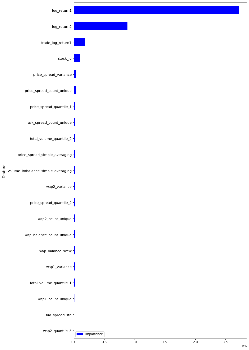
Figure 4. Model feature importance.

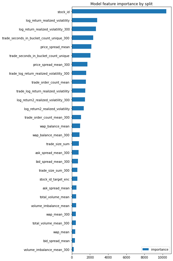
Figure 5. Model feature importance by split.

The related visualization results can be found in Figure 4, Figure 5, Figure 6, Figure 7, Figure 8. The first step of the study employed the LGBM model to examine the importance of model features by split. The results demonstrate that the stock_id parameter exhibited remarkably high importance, surpassing that of the second-ranked parameter, log_return_realized_votaility, by a factor of four. Notably, the majority of parameters evaluated in our analysis displayed an importance value of less than 2000. These findings underscore the crucial role that the stock_id parameter plays in enhancing the model's predictive capabilities in financial markets.

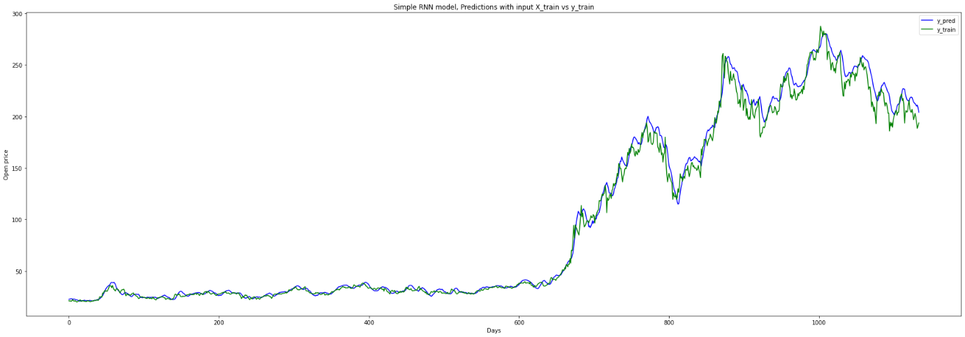
Figure 6. Prediction in a short term.

The RNN model is used to train on a three-year period of stock market data. The findings indicate that the model's predictive performance exhibited close conformity with the training data before 600 days, but began to increasingly deviate from the expected results as the stock market entered a period of oscillation and fluctuation [19]. The phenomenon may be attributed to the RNN model's susceptibility to overfitting, as the model may have learned the idiosyncrasies and patterns of the training data too closely, leading to a reduced ability to generalize to unseen data points.

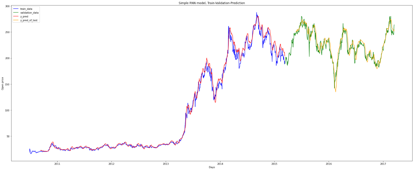
Figure 7. Prediction from 2011 to 2017.

Then the RNN model is applied to a longer period, specifically a five-year period that included both the train and validation sets. The result revealed that during the initial three-year period, which constituted the training set, the model's predictive performance was similar across both the training and validation sets. However, we observed that the model's accuracy on the validation set, which covered the period from 2015 to 2017, showed a modest improvement.

This observed improvement in the model's predictive performance on the validation set may be attributed to several factors [20]. One possible explanation is that the validation set contained more diverse and complex data patterns and trends than the training set, which may have allowed the model to refine its ability to detect and respond to these patterns.

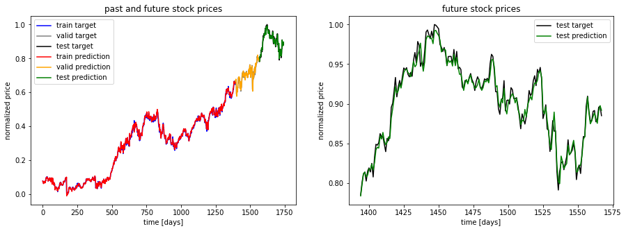
Figure 8. Comparison of stock prices.

In this study, the RNN model was applied to a second 5-year dataset with a distribution of 3.5 years for training and the remaining period for validation and testing. The results demonstrate that the model's performance on the training set was like its performance on the validation and test sets, indicating that the model was able to accurately predict the target variable acmross all periods.

Several factors may have contributed to the model's consistent predictive performance across the different datasets [21]. One possibility is that the model was able to effectively capture the underlying trends and patterns in the data, allowing it to make accurate predictions on both the training and validation/test sets. Additionally, the use of a longer training period may have helped the model to better understand and adapt to the complex patterns and trends present in the data [22].

4. Discussion

Through the feature engineering and development of LGBM, we screened many features of high importance, such as stock ID or logarithmic return 1, and based on the difference of features and the planning of time series, we also re-divided the time series to screen some feature elements at different times, so as to sort out and sort out the social events at that time. It can also be concluded that the style and logarithmic return of stocks in the characteristic project can best reflect the volatility of stock options, which is in line with the capital law of higher risk and greater return. And we found that the important features still include stock ID through secondary analysis for different long or short intervals.

Based on the characteristic engineering analysis, we choose to reduce the dimension of some data to obtain more explicit and effective independent variables for prediction. In the process of using RNN, we increased the number of trainings to obtain more accurate results. It is also found that in the long run, the difference between the forecast effect and the actual data is large, which reversely confirms the uncontrollability and uncertainty of the capital market. In cross validation shown in Table 1, the LGBM model also choose the early stooping to avoid over fitting, the table shows the best iteration.

Table 1. The performance of the model.

Out of folds RMSPE is 0.198322910187951. Finally, this study carried out a cross test with fold of 5 to strengthen the effect of the model, select the optimal parameters and optimize the model, and achieve accurate matching of volatility and returns.

5. Conclusion

In conclusion, this study has proposed a method of predicting the realized volatility of financial assets using LGBM and RNN models. The study has shown that the proposed method can accurately predict the realized volatility of financial assets and can be used to create high returns and achieve the highest sharp ratio. The present dataset has been sourced from a reputable global market maker and can be accessed through Kaggle. The study utilized Convolutional Neural Networks to construct sub-indicators capturing the liquidity and volatility of financial assets, which were used to develop comprehensive measures of liquidity and volatility. Monte Carlo method was applied to solve the integral, which becomes inefficient in the case of high dimension and orthogonality. The study also shows that LGB and other models can efficiently exploit data to create high returns in the current environment.

References

[1]. Koren M Tenreyro S 2007 Volatility and development. The Quarterly Journal of Economics, 122(1) 243-287
[2]. Hnatkovska V 2004 Volatility and growth Vol 3184 World Bank Publications
[3]. Engle R F Patton A J 2001 What good is a volatility model? Quantitative finance 1(2) 237
[4]. Imb J 2007 Growth and volatility Journal of Monetary Economics 54(7) 1848-1862
[5]. Huang D Schlag C Shaliastovich I Thimme J 2019 Volatility-of-volatility risk. Journal of Financial and Quantitative Analysis 54(6) 2423-2452
[6]. Carr P Lee R 2009 Volatility derivatives Annu Rev. Financ. Econ 1(1) 319-339
[7]. Abou O K B 2018 XGBoost and LGBM for Porto Seguro’s Kaggle challenge: A comparison Preprint Semester Project
[8]. Osman M et al. 2021 Ml-lgbm: A machine learning model based on light gradient boosting machine for the detection of version number attacks in rpl-based networks IEEE Access9 83654-83665
[9]. Cai W Wei R Xu L Ding X 2022 A method for modelling greenhouse temperature using gradient boost decision tree. Information Processing in Agriculture 9(3, 343-354
[10]. Kilincer I F Ertam F Sengur A 2022 A comprehensive intrusion detection framework using boosting algorithms Computers and Electrical Engineering 100 107869
[11]. Yin W Kann K Yu M Schütze H 2017 Comparative study of CNN and RNN for natural language processing arXiv preprint arXiv:1702.01923
[12]. Sherstinsky A 2020 Fundamentals of recurrent neural network (RNN) and long short-term memory (LSTM) network Physica D: Nonlinear Phenomena 404 132306
[13]. Yin W Kann K Yu M Schütze H 2017 Comparative study of CNN and RNN for natural language processing arXiv preprint arXiv:1702.01923.
[14]. Williams G Baxter R He H Hawkins S Gu L 2002 A comparative study of RNN for outlier detection in data mining. In 2002 IEEE International Conference on Data Minin Proceedings pp. 709-712 IEEE
[15]. Mao J et al. 2014 Deep captioning with multimodal recurrent neural networks (m-rnn) arXiv preprint arXiv:1412.6632
[16]. Jain A Zamir A R Savarese S Saxena A 2016 Structural-rnn: Deep learning on spatio-temporal graphs. In Proceedings of the ieee conference on computer vision and pattern recognition pp. 5308-5317
[17]. Campos V Jou B Giró-i-Nieto X Torres J Chang S F 2017 Skip rnn: Learning to skip state updates in recurrent neural networks arXiv preprint arXiv:1708.06834
[18]. Keren G Schuller B 2016 Convolutional RNN: an enhanced model for extracting features from sequential data In 2016 International Joint Conference on Neural Networks (IJCNN) (pp. 3412-3419) IEEE
[19]. Peddinti V Chen G Manohar V Ko T Povey D Khudanpur S 2015 Jhu aspire system: Robust lvcsr with tdnns, ivector adaptation and rnn-lms In 2015 IEEE Workshop on Automatic Speech Recognition and Understanding (ASRU) (pp. 539-546) IEEE
[20]. Cho K Van Merriënboer B Gulcehre C Bahdanau D Bougares F Schwenk H Bengio Y 2014 Learning phrase representations using RNN encoder-decoder for statistical machine translation arXiv preprint arXiv:1406.1078
[21]. Mao J Xu W Yang Y Wang J Huang Z Yuille A 2014 Deep captioning with multimodal recurrent neural networks (m-rnn) arXiv preprint arXiv:1412.6632
[22]. Wang J Yang Y Mao J Huang Z Huang C Xu W 2016 Cnn-rnn: A unified framework for multi-label image classification In Proceedings of the IEEE conference on computer vision and pattern recognition (pp. 2285-2294)
Cite this article
An,Z.;Jiang,K.;Zheng,J.R. (2023). Features of realized volatility analysis and return predicting based on LGBM and RNN model. Applied and Computational Engineering,27,38-48.
Data availability
The datasets used and/or analyzed during the current study will be available from the authors upon reasonable request.
Disclaimer/Publisher's Note
The statements, opinions and data contained in all publications are solely those of the individual author(s) and contributor(s) and not of EWA Publishing and/or the editor(s). EWA Publishing and/or the editor(s) disclaim responsibility for any injury to people or property resulting from any ideas, methods, instructions or products referred to in the content.
About volume
Volume title: Proceedings of the 2023 International Conference on Software Engineering and Machine Learning
© 2024 by the author(s). Licensee EWA Publishing, Oxford, UK. This article is an open access article distributed under the terms and
conditions of the Creative Commons Attribution (CC BY) license. Authors who
publish this series agree to the following terms:
1. Authors retain copyright and grant the series right of first publication with the work simultaneously licensed under a Creative Commons
Attribution License that allows others to share the work with an acknowledgment of the work's authorship and initial publication in this
series.
2. Authors are able to enter into separate, additional contractual arrangements for the non-exclusive distribution of the series's published
version of the work (e.g., post it to an institutional repository or publish it in a book), with an acknowledgment of its initial
publication in this series.
3. Authors are permitted and encouraged to post their work online (e.g., in institutional repositories or on their website) prior to and
during the submission process, as it can lead to productive exchanges, as well as earlier and greater citation of published work (See
Open access policy for details).