1. Introduction

Most studies on the impact of monetary policy on investment and consumption are conducted on the transmission channels of monetary policy. Usually, the transmission channels of monetary policy promote economic growth by expanding investment and stimulating consumption through the bank credit market and capital market [1]. One study empirically analyzed data from the United States and found that monetary easing can boost firms' investment activities. Bernanke and Gertler [2] found that monetary policy easing can reduce real interest rates, thus encouraging firms to increase investment. In addition, Kashyap and Stein [3] found that the easing of monetary policy could improve the credit supply capacity of banks and further promote the investment of enterprises.

Another study, using empirical analysis of Chinese data, found that tightening monetary policy had a negative impact on firms' investment decisions. It is found that the tightening of monetary policy may lead to an increase in the real interest rate, thus inhibiting the investment activities of enterprises [4].

As for the impact of monetary policy on consumption, a study conducted by empirical analysis of data from the United States found that monetary policy easing can improve the availability of credit to consumers and promote the increase in consumer spending [5]. The study also found that monetary policy easing can increase consumer confidence levels and further stimulate consumption. However, another study has found that tighter monetary policy can lead to tighter credit and lower consumer confidence, thus depressing consumer spending [3].

There have been some studies on this issue in the existing literature, but there is no systematic and comprehensive analysis, and there are some differences among the research results. This paper uses US GDP data from 1981 to 2022, based on a time series decomposition model with HP filtering, and discusses the impact of monetary policy on investment and consumption through different transmission channels. Based on the results of empirical analysis, this paper will further discuss the effectiveness of current monetary policy on expanding domestic demand on the basis of analyzing the relationship between investment and consumption.

2. Data Description

The dataset under analysis is the U.S. annual real GDP between the years 1981 and 2022, as provided by the U.S. Bureau of Economic Analysis (BEA). It includes the following variables: Personal Consumption Expenditures, Gross Private Domestic Investment, Net Exports of Goods and Services, Government Consumption Expenditures and Gross Investment.

In terms of observations, there are 42 years' worth of data available in the dataset. As the focus of this study is annual GDP, the seasonal component was not considered in this analysis.

3. Model Description

3.1. Time Series Decomposition

First, we briefly described the whole model. Time series can be decomposed into trend components and cyclic components. Since the data in this paper is the annual data of US GDP, its seasonal fluctuations cancel each other out, so the seasonal components are no longer considered. The formula is as follows:

\( GD{P_{t}}={T_{t}}+{C_{t}},t=1,...,T \) (1)

\( {T_{t}} \) represents the trend component, \( {C_{t}} \) represents the cycle component.

Intuitively, if we model \( {T_{t}} \) accurately, then the \( {C_{t}} \) component can be accurately represented as the difference between GDP and the trend component. A linear model was used to model the trend, but there were large errors in the results. Due to the insufficient ability of linear model to describe data, the selection of the model will be biased, so this paper adopts HP filtering to model the trend. The process of HP filtering can be formulated as:

\( \underset{\lbrace {T_{t}}\rbrace }{Min}\lbrace \sum _{t=1}^{T}(GD{P_{t}}-{T_{t}}{)^{2}}+a{\sum _{t=1}^{T}[({T_{t}}-{T_{t-1}})-({T_{t-1}}-{T_{t-2}})]^{2}}\rbrace \) (2)

\( a \gt 0 \) and controls the smoothness of the trend component sequence.

Due to the difference in data frequency choosing quarterly data, choosing annual data in this paper, and improper selection of HP filter parameters will cause distortion of time series [6], so parameter a in HP filter needs to be adjusted. According to paper [7], the smoothing parameter a can be set to 100.

3.2. Evaluation Indicators

After filtering, this paper uses standard deviation, covariance, and goodness of fit of regression of three indicators and draws a co-movement chart to study the impact of consumption and investment on GDP.

Hodrick and Prescott divide the data into two parts and calculate the first half index and the second half index, which further measures the stability of the series [7].

(1) Standard deviation

The sample standard deviations of a series is our measure of a series' variability, which can be formalized as:

\( st{d_{j}}=\sqrt[]{\frac{\sum _{i=1}^{n}({x_{ji}}-{\bar{x}_{j}}{)^{2}}}{n-1}} \) (3)

j means different series.

(2) covariance

The correlation of a series with real GNP is our measure of a series' covariability, which can be formalized as:

\( Cov({X_{j}},GDP)=\frac{\sum _{i=1}^{T}({X_{ji}}-{\bar{X}_{j}})(GD{P_{i}}-\overline{GDP})}{n-1} \) (4)

j means different series.

(3) R2

This paper models the cycle component using the following regression model:

\( {C_{jt}}={a_{j}}+\sum _{i=-2}^{2}{β_{ji}}GD{P_{t-i}} \) (5)

j means different series. then calculate the \( {R^{2}} \) to measure the strength of association with GDP

\( {R^{2}}=1-\frac{\sum ({x_{i}}-\hat{x})}{\sum ({x_{i}}-\bar{y})} \) (6)

(4) co-movement

This indicator can be used to discover the dynamic pattern.

4. Analyze the Impact of Investment and Consumption on GDP

4.1. Indicators

The subsequent research object is changed to a cycle component after the detrending operation. Three indicators are represented to measure the three aspects of the relationships of these three series. The sample standard deviations of a series are the measure of their impact on GDP. The correlation of a series with GDP is the measure of their similarity, which can be viewed in the co-movement figure. R2 is the measure of the strength of association with GDP [7]. All these indicators are computed for the first half and the second half of the sample. This operation can monitor the stability of these indicators over time. This stability can be quantified as a ratio, which ranges from 0 and 1. The closer to 1, the more stable the indicator is (the more correct the regression equation is).The calculation results are shown in the table 1 below:

Table 1: Standard deviations and correlations with GDP

As can be seen from Table 1, in terms of standard deviation, overall Personal consumption expenditures and GDP have very similar standard deviations of 1.75 and 1.74, respectively. But Gross private domestic investment is more than four times GDP. The standard deviation of Personal consumption expenditures is 1.75 as a whole, 1.71 in the first half and 1.83 in the second half, indicating that personal consumption expenditures have a certain impact on the volatility of GDP, and this impact increases in the second half of the time. The standard deviation of Gross private domestic investment is 7.83 as a whole, 7.52 in the first half and 8.3 in the second half, indicating that Gross private domestic investment has a greater impact on the volatility of GDP. It also increased in the second half of the period. Overall, changes in Gross private domestic investment have a greater impact on GDP, whether positive or negative.

For Correlations with GDP, the correlation of Personal consumption expenditures is 0.89 as a whole, 0.86 in the first half and 0.92 in the second half. This indicates that Personal consumption expenditures have a high similarity to GDP, and this similarity increases in the second half of the time. The correlation of Gross private domestic investment as a whole is 0.81, the first half is 0.80, and the second half is 0.78, which indicates that Gross private domestic investment and GDP also have a relatively high similarity. But the similarity decreased slightly in the second half of the time period. Comparing the two shows that both from the perspective of the whole sample and from the perspective of the separate samples, Personal consumption expenditures' correlations are much stronger than Gross private domestic investment. This also shows the pattern that Personal consumption expenditures and GDP have more similar cyclical components, which can be illustrated by Figure 1,2.

From the point of view of stability, whether it is variance or covariance, its changes are relatively small, with good stability.

Table 2: Strength of association with GDP and measure of stability

It can be found in Table 2, when lag and lead GDP are introduced to the regression, the strength of the association of Personal consumption expenditures with GDP decreased from 0.79 to 0.57, and the strength of the association of Gross private domestic investment with GDP increased from 0.66 to 0.78. The Stability Measure of Personal consumption expenditures and Gross private domestic investment is 0.87 and 0.92, respectively. All of them are close to 1, indicating that the regression equations of the two indexes can remain stable with the increase of time.

Based on the above indicators, the standard deviation of consumption is closer to the standard deviation of GDP than that of investment, and the correlation coefficient of investment is larger than that of GDP, indicating that the movement pattern of consumption and GDP is more consistent in the long run. In addition, the parameter window set in the calculation R2 parameter is 5 (years), which measures the impact of components on GDP in the short term. The growth of investment is greater than that of consumption, indicating that investment has a greater impact on GDP in the short term. In summary, the following conclusions can be drawn: (1) Both consumption and investment are positively correlated to GDP, but some investment lags behind at all times. (2) In the long run, consumption has a greater impact on GDP, and in the short run, investment has a greater impact on GDP.

4.2. Co-movement Figure

The co-movement figure of GDP and Personal consumption expenditures and Gross private domestic investment is shown in Figure 1,2:

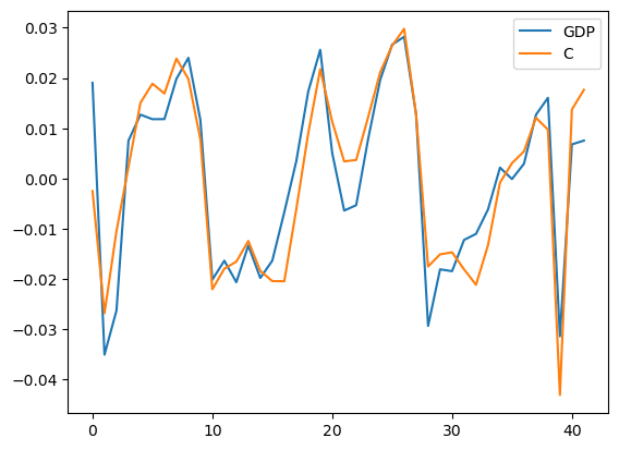
Figure 1: Co-movement figure of GDP and personal consumption expenditures

As can be seen from Figure 1, in general, the synergistic change trends of GDP and Personal consumption expenditures are basically the same, and they are highly similar in detail, but there are also some differences. For example, during the period from 1997 (15) to 1998 (16), The fluctuation of Personal consumption expenditures lags behind that of GDP. The pattern of fluctuations in the time period from 2008 (27) to 2016 (35) is slightly different.

(a) (b)

(c)

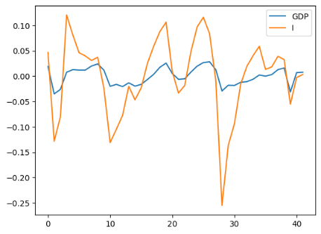
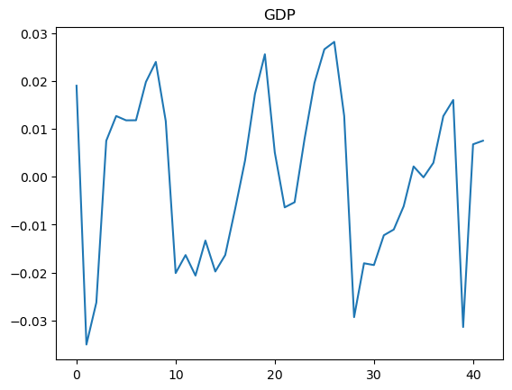
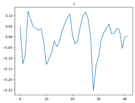
Figure 2: Co-movement figure of GDP and gross private domestic investment (The curves are separated because the variance is too large)

As can be seen from Figure 2, in general, GDP and Gross private domestic investment have obvious differences, and the curve of Gross private domestic investment is smoother than that of GDP. Taking 1996 (15) as the limit, the fluctuation patterns of GDP and Gross Private Domestic Investment before 1996 were significantly different, and they were more similar after 1996.

5. Analyze

5.1. Theoretical Analysis

In the short term, monetary policy may impact the borrowing behavior of businesses and individuals by changing market interest rates. For instance, if the central bank lowers the benchmark interest rate, the interest rates that commercial banks offer to businesses and individuals may also decrease. This makes loans more affordable, thereby encouraging businesses to invest and individuals to consume. That is, it leads to an increase in GDP by promoting consumption/investment. For example, companies may choose to borrow to invest in new production equipment, and individuals may choose to borrow to purchase cars or property. The increase in these investments and consumption directly drives the growth of GDP (Figures 1, 2). Conversely, if the central bank raises the benchmark interest rate, the cost of loans will increase, potentially suppressing business investment and personal consumption, thereby affecting the growth of GDP. Furthermore, in Figure 2, we can see that investment and GDP generally show a positive correlation, but from 1991 (10) to 1999 (18), the rise in investment did not immediately lead to a significant increase in GDP, which could be due to information or effect lags in monetary policy.

In the long run, the influence of monetary policy on investment, consumption, and GDP is more complex. On the one hand, a moderate money supply and low-interest rates can help businesses and individuals increase investment and consumption. On the other hand, excessive money supply may lead to inflation. High inflation raises the cost of production and living, which may suppress business investment and personal consumption. Moreover, high inflation can cause economic instability, which is also detrimental to investment and consumption.

For instance, in Figures 1 and 2, we can see that GDP and consumption, GDP and investment, present an economic cycle of approximately 10 years. This is because central banks or other monetary authorities indeed adjust monetary policy according to changes in economic conditions, aiming to stabilize the economy, control inflation, and maintain employment, among other goals. From the perspective of monetary policy, when the economy overheats, policymakers might use contractionary monetary policy, such as raising interest rates, to prevent excessive inflation. Under this policy, when the economy gradually shows signs of recession, policymakers might use expansionary monetary policy, such as lowering interest rates or implementing quantitative easing, to stimulate economic activity and prevent too high unemployment, thereby presenting a cyclical pattern in the chart.

5.2. Case Study

After the global financial crisis in 2008, the U.S. Federal Reserve (Fed) took unprecedented monetary policy measures to stimulate the economy, namely quantitative easing. The primary measure of this policy was to lower the federal funds rate to near zero levels and buy a large number of long-term Treasury bonds and mortgage-backed securities to increase the cash supply in the banking system, lower long-term borrowing rates, and encourage investment and consumption. This impact can be observed in the data after the 2008 (26) point in Figure 2, where investment and consumption both increased, and the economy showed a trend of recovery.

This policy had significant short-term effects. Due to the substantial reduction in loan interest rates, both businesses and individuals were more willing to borrow for investment and consumption, which greatly stimulated the recovery of the U.S. economy. For instance, low-interest rates made loans for the real estate market cheaper, encouraging more people to buy homes and thus stimulating the recovery of the real estate market.

However, in the long run, this policy also brought some problems. First, a large amount of money supply could trigger inflation. Although the U.S. did not experience significant inflation at the beginning of the crisis, inflationary pressure began to emerge in the following years. Second, excessively low-interest rates might encourage over-investment and the accumulation of debt, thereby leading to asset bubbles. For example, excessively low-interest rates could lead businesses and individuals to over-borrow, causing debt problems. At the same time, excessively low-interest rates could also drive up prices in the stock market and real estate market, forming asset bubbles.

6. Conclusion

Monetary policy, implemented by central banks, uses tools such as adjusting money supply, interest rates, and exchange rates to attain economic goals like price stability and growth. Its impact on investment primarily works through two channels: interest rate and credit. The central bank's monetary policy also impacts consumption by adjusting policy interest rates and thus affecting the cost of loans and savings. Increased rates can make consumers and businesses cautious about borrowing, reducing consumption and slowing down economic activity.

In short, monetary policy further affects GDP by affecting investment and consumption. This paper reveals the impact of consumption and investment on GDP, and then explains the impact of monetary policy on GDP

The first section of the study focuses on evaluating the influences of investment and consumption on GDP. This analysis considers the detrended cyclical components of GDP, investment, and consumption. Various measures are utilized to understand these relationships. Standard deviations offer a measure of the impact each series has on GDP, correlations provide a similarity measure, and R-squared values indicate the strength of the association with GDP. These metrics are computed for both the first and the second halves of the sample, enabling a comparative analysis of their stability over time.

Results from these calculations underscore some noteworthy patterns. Personal consumption expenditures have a high correlation with GDP, indicating they have similar cyclical components. Conversely, the standard deviation of gross private domestic investment is significantly higher than that of GDP, suggesting that changes in investment have a more profound impact on GDP volatility.

The stability measures obtained from both variance and covariance calculations exhibit minimal change, implying an overall stability in the metrics. Co-movement figures or graphs, demonstrating the alignment in GDP with personal consumption expenditures and gross private domestic investment, substantiate these findings. They reveal a higher similarity in the change trends of GDP with personal consumption expenditures, despite some minor differences. Comparatively, GDP and Gross private Domestic investment portray more considerable differences, with the latter presenting a smoother curve.

The second of study reveals that monetary policy plays a critical role in influencing economic behavior and outcomes, both in the short and long term. In the short term, adjustments in interest rates can effectively impact the borrowing behavior of businesses and individuals, thereby stimulating or moderating consumption and investment and, subsequently, influencing GDP growth. However, the effects may not always be immediate due to possible lags in information or policy impacts.

Over the long run, the dynamics become more complex. While a moderate money supply and low interest rates can foster economic growth by promoting investment and consumption, an excessive supply of money can lead to inflation and economic instability. These conditions can, in turn, discourage investment and consumption, potentially undermining economic growth and stability.

The case of the U.S. Federal Reserve's response to the 2008 financial crisis underscores the potency of monetary policy tools like quantitative easing in stimulating economic recovery in the short term. However, it also highlights the potential pitfalls of such policies over the long term, including inflationary pressures and the risk of creating asset bubbles through over-investment and debt accumulation.

Therefore, it is crucial for policymakers to strike a delicate balance when implementing monetary policies. They must remain responsive to short-term economic conditions while also being cognizant of the long-term implications to ensure sustainable economic growth and stability.

In conclusion, this comprehensive analysis offers valuable insights into the cyclic components of the GDP series and the influences of investment and consumption on GDP, highlighting the different patterns exhibited by consumption and investment in relation to GDP and how monetary policy affects GDP. This study, therefore, serves as a vital resource for economists and policy-makers, empowering them with a more nuanced understanding of the dynamics at play within the economy.

References

[1]. Jean, B., Michael, T, K., Frederic, S, M., (2011). How Has the Monetary Transmission Mechanism Evolved Over Time? Handbook of Monetary Economics.
[2]. Bernanke, B. S., Gertler, M. (1995). Inside the black box: The credit channel of monetary policy transmission. Journal of Economic Perspectives, 9(4), 27-48.
[3]. Kashyap, A. K., & Stein, J. C. (1995). The impact of monetary policy on bank balance sheets. Carnegie-Rochester Conference Series on Public Policy, 42, 151-195.
[4]. Christiano, L. J., Eichenbaum, M., & Evans, C. L. (1996). The effects of monetary policy shocks: Evidence from the flow of funds. Review of Economics and Statistics, 78(1), 16-34.
[5]. Romer, C. D., & Romer, D. H. (2004). A new measure of monetary shocks: Derivation and implications. American Economic Review, 94(4), 1055-1084.
[6]. Schüler, Y, S., (2018). Detrending and financial cycle facts across G7 countries: Mind a spurious medium term!
[7]. Hodrick, R, J., Prescott, E, C., (1997). Postwar US business cycles: an empirical investigation. Journal of Money, credit, and Banking: 1-16.
Cite this article
Zhang,Z. (2024). The Effects of Monetary Policy on Investment and Consumption——Taking the US GDP Data from 1981 to 2022 as an Example. Advances in Economics, Management and Political Sciences,73,299-306.
Data availability
The datasets used and/or analyzed during the current study will be available from the authors upon reasonable request.
Disclaimer/Publisher's Note
The statements, opinions and data contained in all publications are solely those of the individual author(s) and contributor(s) and not of EWA Publishing and/or the editor(s). EWA Publishing and/or the editor(s) disclaim responsibility for any injury to people or property resulting from any ideas, methods, instructions or products referred to in the content.
About volume
Volume title: Proceedings of the 2nd International Conference on Financial Technology and Business Analysis
© 2024 by the author(s). Licensee EWA Publishing, Oxford, UK. This article is an open access article distributed under the terms and
conditions of the Creative Commons Attribution (CC BY) license. Authors who
publish this series agree to the following terms:
1. Authors retain copyright and grant the series right of first publication with the work simultaneously licensed under a Creative Commons
Attribution License that allows others to share the work with an acknowledgment of the work's authorship and initial publication in this
series.
2. Authors are able to enter into separate, additional contractual arrangements for the non-exclusive distribution of the series's published
version of the work (e.g., post it to an institutional repository or publish it in a book), with an acknowledgment of its initial
publication in this series.
3. Authors are permitted and encouraged to post their work online (e.g., in institutional repositories or on their website) prior to and
during the submission process, as it can lead to productive exchanges, as well as earlier and greater citation of published work (See
Open access policy for details).