1. Introduction

The COVID-19 pandemic has had significant effects on the global economy, leading to an economic recession in many countries. In April 2021, the U.S. unemployment rate shot up to 14.7 percent [1], while personal consumption expenditures were almost 20 percent lower than at their peak.

The pandemic has resulted in a significant economic recession, affecting various aspects of the economy and governments have taken measures to mitigate the economic impact. But the recovery process remains uncertain and depends on factors such as vaccine distribution and the containment of the virus. Hence, a convincing prediction made to the economics data during the recession is of importance since it provides basis for policy-makers to taking effective action.

While there are a range of forecasting methods used by different section in society, many of them are less effective when it comes to recession. According to Marcelle Chauvet and Simon Potter [2], though DSGE models, VAR models, and BVAR models are commonly used during the normal time, they are outperformed by simple autoregressive AR (2) models and all of them are less efficient. Besides, in the other article by Giorgio E. Primiceri and Andrea Tambalotti [3], The writers identify the problem that the forecasting method involving time-series model is lacking for parallel historical data of a Shock in history. On the other hand, more structural models are complicated with assumption.

Although many of traditional model are less reliable during recession time, a few of articles make use of machine learning to make prediction. Machine learning shades a light for predicting data that bears complicated but implicit effect, which is hardly to define in a formulated way. Hence, the method is widely used in Macroeconomics research like AS Hall [4] finds it better than statistical approach in terms of complexity, where machine learning can find the optimal complexity for model to balance biasness and variance. Apart from the simplicity for user to get started, the accuracy of forecasting by machine learning is outstanding. Jaehyun Yoon [5] has made forecasting on GDP data in Japan with random forest and gradient boosting, which turns out a better performance comparing with the forecasts by the International Monetary Fund and Bank of Japan. Nyman and Paul [6] make use of random forest algorithm to make prediction involving data from financial crisis in 2008. In both United kingdoms and United states, though machine learning algorithm cannot foresee the emergence of a recession, it still performed better than time series models. Besides, Sima Siami-Namini, Neda Tavakoli and Akbar Siami Namin [7] made a comparison between time-series model and cutting-edge deep learning model Long-short term memory (LSTM), where the empirical studies conducted and reported in this article show that deep learning-based algorithms such as LSTM outperform traditional-based algorithms such as ARIMA model.

This article aims to examine the performance of some commonly-used model during the recession time. In the first section, a board range of forecasting models will be introduced including time-series model VAR, machine learning models and deep learning model. In the empirical part, the performance of these model will be carefully examined in empirical analysis on pandemic data in United States America. Given the purpose of trying to compare the performance of models, techniques that contribute to improve the predicting power will be used such as cross-validation to check the optimum performance. The empirical outcome provides the evidence on the performance of models during the recession time and shades light on further more accurate forecasting on the economic recession.

2. Predictive Model

2.1. Data Summary

To select the most significant features to be fed into prediction model, some features commonly used in predicting models are primarily selected. The features pool is comprised of Gross domestic product (GDP), unemployment rate (unemployment), Producer price index (PPI), Housing price index, Total population (population), NASDAQ stock market index (NASDAQ), interest rate of 1-year treasury bill (Treasury bill rate), interest rate of corporate bonds (Corporate bonds rate), Net export and federal saving rate (saving rate). All of the features are quarterly recorded by Statistics Bureau of USA and range from the first quarter in 1973 to the second quarter in 2023, with 161 samples in total.

Among the features, most of them are with increasing trend except for unemployment, treasury bill rate and corporate bonds rate. The interest rate of treasury bill and corporation bonds are decreasing with sharp fluctuation whereas unemployment rate sharply fluctuates periodically without explicit trend. Besides, PPI, NASDAQ and housing price index shows variation to some extend and there are outstanding peaks and bottom in some period, corresponding for events with large impact. The GDP and population are smoother in the whole range of time.

Table 1: Descriptive statistic for US data

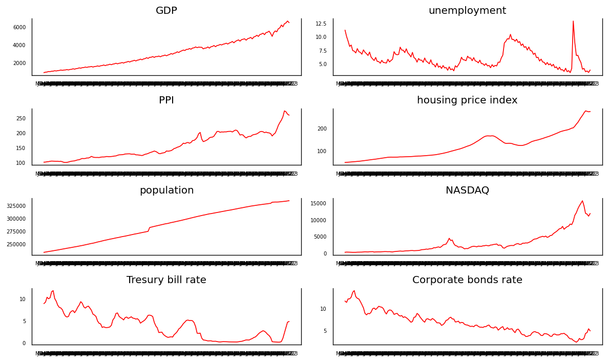
Figure 1: Data path for US

2.2. Empirical Models

When making forecasting, this article use both time series model and machine learning models for forecasting. The former one merely involves Vector autoregression (VAR) model whereas the latter contains Support Vector Regression (SVR), Gradient Boost Regressor, eXtreme Gradient Boost Regressor (XGboost) and Long-short term Memory (LSTM).

To make sure obtaining the best predicting performance, feature selection is conducted before constructing each model. For the dataset provided, the predictors fed into model is a subset of overall features, where it requires carefully selecting the predictors that generates best forecasting performance. The vary technique applied for features selection is Recursive Features Elimination (RFE). The Recursive Feature Elimination (RFE) works by recursively removing attributes and building a model on those attributes that remain. By explicit defining the number of features a model required, RFE produce the combination of features with best performance or minimum prediction error in a specific model. When stepping forward to automatically select the number of features, RFE can be alloyed with cross-validation on the number of features, which can be achieved with RFECV module in scikit-learn in python.

Along with RFE, after the features are defined, cross-validation process is used to tune the parameters and get avoid to overfitting problems. For all the models, data first is split into training set and test set, where the former serves for fitting model and the latter is used to make prediction. Given the data set has limited sample, k-fold cross-validation works well for tuning parameters. It simply further split the training set into K section and conducting predict-test process K times. The optimal parameter is obtained from these outcomes. In python, cross-validation process can be achieved by GridSearchCV by specify the range of hyperparameter. In this article, mean squared error is used for scoring the performance of model and set folding number k = 10. The overall optimal hyperparameter for models are summarized in table 4.

2.2.1. Vector Autoregression (VAR)

Vector Autoregression (VAR) is a forecasting algorithm that can be used when two or more time series influence each other. That is, the relationship between the time series involved is bi-directional. in general, a pth-order VAR refers to a VAR model which includes lags for the last p time periods. A pth-order VAR is denoted "VAR(p)" and written as

\( {Y_{t}}=C+{A_{1}} {Y_{t-1}}+{A_{2}} {Y_{t-2}}+…+{A_{q}} {Y_{t-q}}+{e_{t }}\ \ \ (1) \)

The first step for modelling is to eliminate the features being less likely correlated with GDP data. To determine the relationship, the article conduct Granger’s causality test to test the causality between features. Granger’s causality tests the null hypothesis that the coefficients of past values in the regression equation is zero. By feeding the data, causality test produces an outcome matrix with p-value showing in following table.

Table 2: Causation matrix for US data

Since the model is to predict GDP, it's reasonable to focus on the result of the function with GDP being dependent variable. The result of causation test shows that there is no enough evidence to reject the coefficient of corporate bonds rate being zero whereas the other variables are correlated with GDP data of US. We then eliminate corporate bonds rate from the model for US. Result for Italy data shows all variables are correlated with GDP data, which suggest no features will be eliminated.

Secondly, like many time-series model, VAR model implicitly require stationarity for each of the features. Therefore, Augmented Dicky-Fuller test (ADF test) is used whose null hypothesis is that a unit root presents in series, which means the underlying series is non-stationary. By taking the test, finally differenced all series by 1 time and all series become stationary.

The final step is to determine the lagged times or q’s value in VAR(q). To optimized the performance of model, one may select the model with least prediction error. One way for optimizing the performance is based on criterion indicating the prediction error. The article take use of Akaike information criterion (AIC) and Bayesian information criterion (BIC), both of which are indicating the prediction error and thereby the quality of statistical model given a set of data. The smaller the criterion, the less the prediction error. According to the result, AIC keep decreasing as q increases and BIC firstly increase and falls sharply in q = 3, with increasing from then on for US data.

2.2.2. Support Vector Regression (SVR)

Support Vector Regression shows advantage in conducting regression problem. The idea of SVR comes from Support Vector Machines (SVMs), which was first identified by Vladimir Vapnik and his colleagues in 1992 and widely used in classification problem. The idea of SVMs is to find a hyperplane to classify data in a higher dimension with the help of kernel function and decision boundary severing as ignorance of error [8]. Whereas SVR serves for regression problem, where it tries to find a function that approximates the relationship between the input variables and a continuous target variable, while minimizing the prediction error. What makes it better than simple linear regression is that SVR can not only handle non-linear relationships between the input variables and the target variable by using a kernel function to map the data to a higher-dimensional space but tolerate error terms with the help of decision boundary, making it more flexible when dealing with different dataset.

In SVR, the underlying hyperparameter for tuning consist of kernel function with ‘linear’, ‘polynomial’ and ‘rbf’ for considering, epsilon ranging from 0.01 to 0.5 and regulation from 1 to 20.

2.2.3. Gradient boosting Machine (GBM)

Gradient boosting Machine is established for its accuracy for classification and regression task. Since it was first introduced by Leo Breiman, amount of works of forecasting in Economics and financial field are conducted based on the vary machine learning algorithm.

The idea of Gradient boosting Machine for regression task begin with creating a single leaf that represents an initial guess for all samples. It then built a tree with restricted length based on the error of tree (leaf) made before. With scaling each tree by the same amount, GBM create trees until a set number or when additional tree can not improve the overall performance. It’s noticed that trees in GBM are predicting the residual thus the final value being produced by sum of initial guess and the result of all trees. Besides, by getting off over-fitting problem, each tree has a learning rate between 0 to 1 to constrain the outcome of each tree. Mathematically speaking, GBM for regression takes following steps:

ALGORITHM 1: Gradient boost Algorithm

Input

: \( Data\lbrace ({X_{i}},{Y_{i}})\rbrace ,for i=1…n and a differentiable loss function L({y_{i}},F(x)) \)

Step 1: initialize model with a constant value:

\( {F_{0}}(x)={argmin_{γ}}\sum _{i=1}^{n}L({y_{i}}, γ) \)

where \( yi \) is an observed value, and \( γ \) is a predicted value. \( {F_{0}}(x) \) is the average of the observed values.

Step 2: For m=1 to M:

Compute

\( {γ_{im}}=-{[\frac{∂L({y_{i}},F({x_{i}}))}{∂F({x_{i}})}]_{F(x)={F_{m-1}}(x)}}, For i=1…n \)

(B) Fit a regression tree to the \( {γ_{im}} \) values and create terminal regions \( {R_{jm}} for j = 1 …Jm \) .

I For j = 1 …Jm, compute

\( {γ_{im}}={argmin_{γ}}\sum _{{x_{i}}∈{R_{ij}}}L({y_{i}},{F_{m-1}}({x_{i}})+ γ) \)

(D) update

\( {F_{m}}(x)= {F_{m-1}}(x)+v\sum _{j=1}^{jm}{γ_{im}}I ({x_{i}}∈{R_{jm}}) \)

Step 3: output \( {F_{m}}(x) \)

When forecasting GDP data in this article, same features selection method RFECV on training set is conducted on the vary beginning. After obtaining the combination of predictors, k-fold cross validation is conducted for tuning the parameter containing learning rate ranging from 0.01 to 0.2, number of trees ranging from 100 to 500, maximum length of tree in 10 and minimum split in a tree within 10.

2.2.4. eXtreme Gradient Boosting (Xgboost)

Since it is Introduced firstly in 2016 by Chen and Guestrin, Xgboost received greatly reputation for its efficiency and computation speed. Xgboost follows the principle of boosting that contains several weak learners such that each weak learner can contribute a small improvement to prediction. While both Xgboost and gradient boosting shares the same gradient boosting principle, Xgboost build the decision tree based on similarity score thereby a corresponding gain value.

The regularization term aims to reduce the likelihood of overfitting by controlling the complexity of constructed trees. The complexity of each tree follows the equation:

\( Ω(f)= γT + \frac{1 }{2} λ \sum _{j=1}^{T}w_{j}^{2}\ \ \ (2) \)

where T is the number of leaves and ω is the vector scores on leaves. The structure score, objective function, of the algorithm is defined as:

\( F = \sum _{j=1}^{T}({G_{j}}{w_{j}}+\frac{1}{2}({H_{j}}+λ)w_{j}^{2})+γT\ \ \ (3) \)

where \( ωj \) are independent from each other and the form \( \sum _{j=1}^{T}({G_{j}}{w_{j}}+\frac{1}{2}({H_{j}}+λ)w_{j}^{2} \) is quadratic.

When forecasting GDP data in this article, same features selection method RFECV on training set is conducted on the very beginning. After obtaining the combination of predictors, k-fold cross validation is conducted for tuning the parameter. The hyperparameters for tuning contains round referring to the maximum number of trees made, learning rate from 0 to 0.2, maximum length for each tree from 1 to 10, the complexity parameter gamma that used to prune the tree ranging from 0 to 0.9 and regularization parameter lambda that used to reduce the influence of a single value to get rid of over-fitting ranging from 0 to 5. Cross-validation process select the parameter set based on training set that produce least mean absolute error thereby the best performance.

2.2.5. Long-Short Term Memory (LSTM)

Long-short term memory is a kind of Recurrent Neural Network (RNN) that make use of sequence of earlier data to make future prediction. While RNN allows sequential input to feed into model to make prediction with the help of a loop, it is seldomly used in practical to make forecasting. The reason is the exploding/vanishing gradient problem occurs when large sequence of data is trained to RNN. That’s when large sequence of past data is used to predict future data, the effect of earliest data will be exploded or vanished depending on the value of weight which makes it ineffective in practice.

To solve the problem of exploding/vanishing gradient, LSTM is designed for predict large sequence of data. In LSTM, long-term memory or cell state flows all neurons without weight or bias directly affecting and short-term memory or hidden state are adjusted in each neuron by inputs and cell state. When LSTM works, each neuron first received a hidden state propagated by last neuron and an input value. It then determines what percentage of cell state need to be preserved. The process is named ‘forget gate’ and then pass to ‘input gate’. Input gate helps to create a potential long-term memory and decide what percentage of the potential memory is added into cell-sate. Followed by an ‘output gate’, it then produces a new hidden-sate or short-term memory at the end of a neuron which passed to next neuron. Due to the use of some gates in each cell, data in each cell can be disposed, filtered, or added for the next cells and hence the prediction is more precise in many of empirical research.

In this article, GDP data is used to make time-series forecasting where multi time steps are used to make prediction of next time steps which is so called window approach. And the number of time steps used for prediction is a parameter to be decides. A function is being created to decides the parameter based on the performance of forecasting with data in training set which is achieved by recursively run the model with data containing different set of series and find the group producing least mean square error.

By obtaining the number of time steps, then we decide the parameters Epoch and batch for finding best model. Epoch is the number the data run through the network, which set from 100 to 300, and batch is the parts data platting, which is set from 1 to 4.

Table 3: Hyperparameters for Models

2.3. Model Predictions

All the model for same country shares the same data pools defined in previous part except for LSTM model in which a dataset only containing GDP data of difference lagged time is created. To get rid of over-fitting problem which is described as the model fit too good to training data to make an unbiased prediction, overall dataset is split into a training set and a test set with the help of train-test-split module in python. Where the training set is used for fitting the model and tuning the parameter by k-fold cross-validation and test set is used for make prediction and overview the performance of each model. The test size is set for 25% of total sample size. For VAR model, the test size is only for 4 quarters since it’s for short-run prediction.

The overall performance of model is measured by assessment matrix. The Root-Mean-Square Error (RMSE) is a commonly employed metric for evaluating the accuracy of predictions generated by a model. It calculates the discrepancies or residuals between the actual and predicted values. This metric is used to compare the prediction errors of various models for a specific dataset, rather than between different datasets. Mean Absolute Error (MAE) represents the average of the absolute differences between predictions and actual observations over the test sample. The formula for computing RMSE and MAE is as follows:

\( RMSE= \sqrt[]{\frac{1}{N}\sum _{i=1}^{N}{({x_{i}}-\hat{{x_{i}}})^{2}}} \ \ \ (4) \)

\( MAE= \frac{1}{N}\sum _{i=1}^{N}|{x_{i}}-\hat{{x_{i}}}|\ \ \ (5) \)

According to the result shown in following table, Extreme Gradient Boost has an RMSE of 100.7132 and an MAE of 73.0465, indicating relatively accurate predictions with low errors. Long-Short Term Memory has an RMSE of 127.5657 and an MAE of 69.6715. While the MAE is slightly lower than that of XGBoost, the RMSE is higher, suggesting that LSTM may have a few larger errors in its predictions. SVR has the highest RMSE and MAE values among the models, with an RMSE of 191.7369 and an MAE of 156.4849. This implies that the SVR model's predictions are less accurate compared to the other machine learning models. Gradient Boost has a performance similar to XGBoost, with an RMSE of 98.3748 and an MAE of 73.3277. This suggests that Gradient Boost is also a strong predictor of quarterly GDP data. Vector Autoregression (VAR(3)) has the highest RMSE and MAE values, at 674.1517 and 667.3426, respectively which indicates that the VAR(3) model's predictions are less accurate than those of the other models.

Three machine learning models outperform to time-series model VAR(q) to a large extend. Among models, the Gradient Boost and Extreme Gradient Boost models appear to have the best performance in forecasting quarterly GDP data in the United States. The Long-Short Term Memory (LSTM) model also shows promising results, while the Support Vector Regression (SVR) and Vector Autoregression (VAR(3)) models perform less accurately in comparison to the other models.

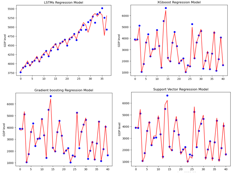
Figure 2: Forecasting result for US

3. Limitations of Model

In this article, models involve time-series forecasting, machine learning algorithm and deep learning are used to make forecasting based on the decades data involving the data in pandemic. Although the result of models provides evidence on the performance of models during the recession time, it is far from a practical now-casting data. The data set is basically range several decades and collected seasonally, which on one hand affect the accuracy of model when predicting the recession and on the other hand is lacking information given the recession usually is of sharpness and sudden. In most of the article focus on recession, now-casting is the exercise of reading, through the lenses of a model, the flow of data releases in real time, in which more frequent data like daily data and mixed-frequency data are used in order to provide real-time and flexible forecasting, which is of more practical to make policy. But this is beyond the bound of this article.

4. Conclusion

This article deals with forecasting method on Macroeconomics variables in recession period of covid-19. The purpose of article is to examine the performance of machine learning algorithm during the recession period. The article firstly addresses the framework of recession and check the correlation based on the process of VAR model between economic data. It then introduces and compares three popular machine learning methods: support vector regression, gradient boosting and extreme gradient boosting. Besides, time-series forecasting model VAR and deep learning algorithm LSTM are introduced as well. Next, to make sure obtaining the best predicting performance, feature selection is conducted before constructing each model by the technique Recursive Features Elimination (RFE). Along with RFE, after the features are defined, cross-validation process is used to tune the parameters and get avoid to overfitting problems. The article conducts empirical analysis based on the models built in previous part and stress on whether the model perform well by involving the recession data and makes a comparison among these models. US data from 1973 to 2023 are used to make sure important recessions are contained. The result indicates that machine learning algorithm are all well performed in US where they generate relatively low forecasting error. Among models, the Gradient Boost and Extreme Gradient Boost models appear to have the best performance in forecasting quarterly GDP data in the United States.

References

[1]. Heather, L., Andrew, V.D. (2020) U.S. unemployment rate soars to 14.7 percent, the worst since the Depression era. The Washington Post, Retrieved from https://www.washingtonpost.com/business/2020/05/08/april-2020-jobs-report/
[2]. Chauvet, M., & Potter, S. (2013). Forecasting output. Handbook of economic forecasting, 2, 141-194.
[3]. Primiceri, G. E., & Tambalotti, A. (2020). Macroeconomic Forecasting in the Time of COVID-19. Manuscript, Northwestern University, 1-23.
[4]. Hall, A. S. (2018). Machine learning approaches to macroeconomic forecasting. The Federal Reserve Bank of Kansas City Economic Review, 103(63), 2.
[5]. Yoon, J. (2021). Forecasting of real GDP growth using machine learning models: Gradient boosting and random forest approach. Computational Economics, 57(1), 247-265.
[6]. Nyman, R., & Ormerod, P. (2017). Predicting economic recessions using machine learning algorithms. arXiv preprint arXiv:1701.01428.
[7]. Siami-Namini, S., Tavakoli, N., & Namin, A. S. (2018, December). A comparison of ARIMA and LSTM in forecasting time series. In 2018 17th IEEE international conference on machine learning and applications (ICMLA) (pp. 1394-1401). IEEE.
[8]. Cortes, Corinna; Vapnik, Vladimir (1995). "Support-vector networks", Machine Learning. 20 (3): 273–297.
Cite this article
Yu,M. (2024). Machine Learning for Economic Forecast Based on Past 30 Years and Covid-19 Pandemic Data. Advances in Economics, Management and Political Sciences,80,129-138.
Data availability
The datasets used and/or analyzed during the current study will be available from the authors upon reasonable request.
Disclaimer/Publisher's Note
The statements, opinions and data contained in all publications are solely those of the individual author(s) and contributor(s) and not of EWA Publishing and/or the editor(s). EWA Publishing and/or the editor(s) disclaim responsibility for any injury to people or property resulting from any ideas, methods, instructions or products referred to in the content.
About volume
Volume title: Proceedings of the 3rd International Conference on Business and Policy Studies
© 2024 by the author(s). Licensee EWA Publishing, Oxford, UK. This article is an open access article distributed under the terms and
conditions of the Creative Commons Attribution (CC BY) license. Authors who
publish this series agree to the following terms:
1. Authors retain copyright and grant the series right of first publication with the work simultaneously licensed under a Creative Commons
Attribution License that allows others to share the work with an acknowledgment of the work's authorship and initial publication in this
series.
2. Authors are able to enter into separate, additional contractual arrangements for the non-exclusive distribution of the series's published
version of the work (e.g., post it to an institutional repository or publish it in a book), with an acknowledgment of its initial
publication in this series.
3. Authors are permitted and encouraged to post their work online (e.g., in institutional repositories or on their website) prior to and
during the submission process, as it can lead to productive exchanges, as well as earlier and greater citation of published work (See
Open access policy for details).