1. Introduction

In contemporary society, automobiles stand as one of the most integral and convenient modes of transportation, often chosen by many for their travel needs. The analysis and prediction of new and used car sales emerge as pivotal elements, carrying substantial implications across diverse economic landscapes. Such insights prove invaluable to both suppliers and consumers, fostering a more profound comprehension of the automotive sales market dynamics.

This research delves into the application of SARIMA models, a promising avenue for understanding and forecasting sales trends. By employing SARIMA models on two distinct time series, this study aims to predict future sales, shedding light on the accuracy of short-term forecasts. This dual-pronged approach not only facilitates sellers in formulating effective sales strategies but also empowers buyers to make informed purchasing decisions.

An integral component of contemporary business intelligence is sales forecasting [1]. Sales forecasting is recognized as a complex challenge, wherein accurate predictive models assist businesses in uncovering potential risks and making more informed decisions [2,3]. Forecasts hold significance in the automotive industry, as precise predictions can effectively reduce inventory buildup, prevent missed sales opportunities, and mitigate issues of over-supply [4,5].

Simultaneously, several studies have successfully employed SARIMA models for real-time series analysis and forecasting [6-10]. These studies underscore the significance of sales forecasting and the feasibility of SARIMA models for real-time series prediction.

This paper conducts a comprehensive time series analysis of new and used car sales in the United States, selecting SARIMA models based on standards such as AICc, RMSE, MAE, and MAPE. The subsequent forecasting of sales for the upcoming two years aims to provide a robust understanding of the market dynamics and trends, contributing to both academic discourse and practical applications within the automotive industry.

2. Methodology

2.1. Description of Data

The dataset used in this study is sourced from the United States Census Bureau (http://www.census.gov/), consisting of monthly figures for new car sales and used car sales. The data spans from January 1992 to November 2023 and is presented in Figure 1. For new car sales, the trend shows fluctuating increases, but experienced significant declines around 2009 and 2022, respectively. Similarly, for used car sales, the overall trend is characterized by fluctuating increases, with substantial declines in the same years. However, compared to the sales of new car, the monthly sales and volatility are lower for used car.

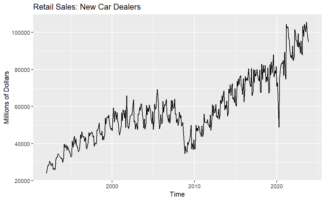
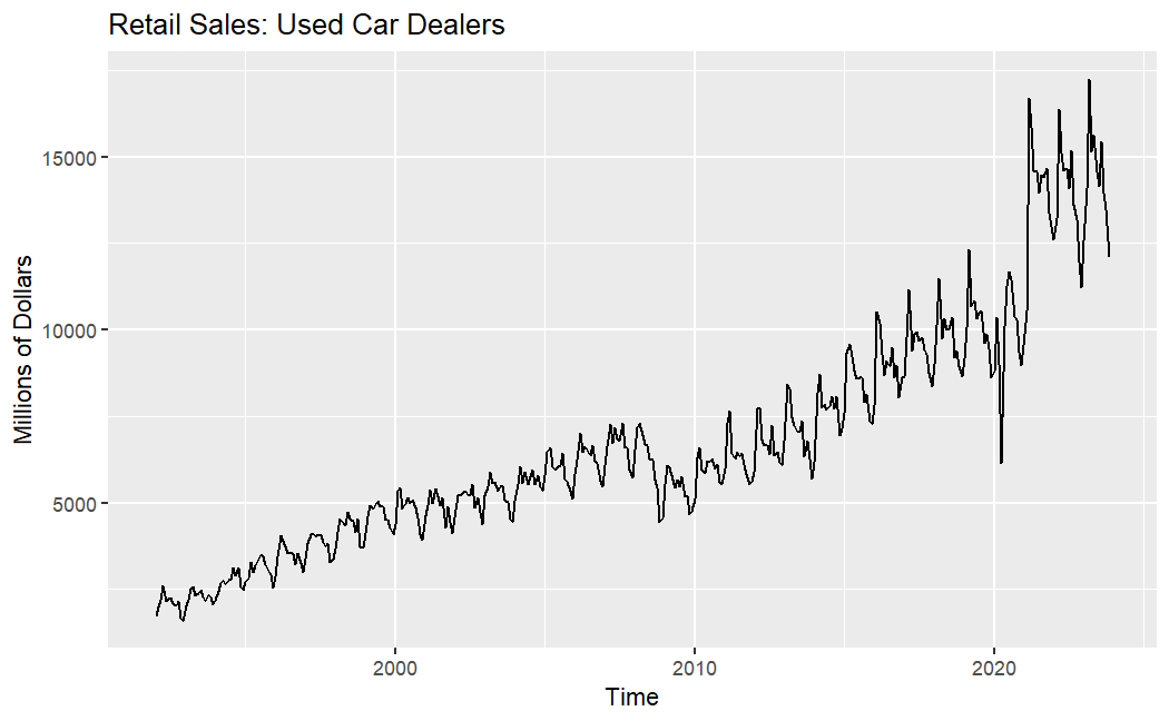
(a) New car (b) Used car

Figure 1: Retail sales for new car(a) and retail sales for used car (b).

2.2. Time Series Patterns Analysis

To better fit models later, now conduct an analysis of these time series. From Figure 2, it can be observed that for new car, retail sales increase slightly in February, then fluctuates. For used car, retail sales rise in February and March, then slowly declines.

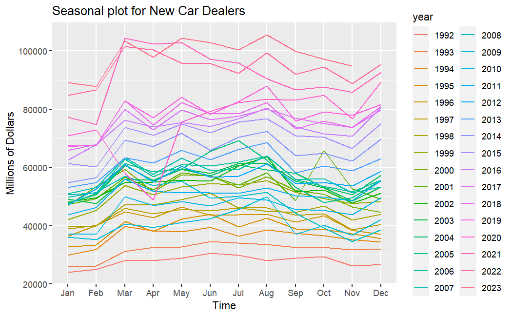
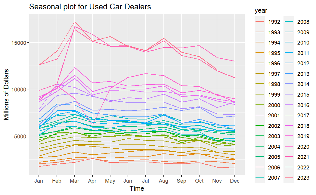
(a) New car (b) Used car

Figure 2: Seasonal plot for new car sales(a) and used car sales(b).

Figure 3 further illustrates the trends in the data, and it is evident that the trends of these time series are clearly visible.

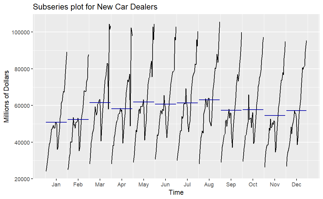
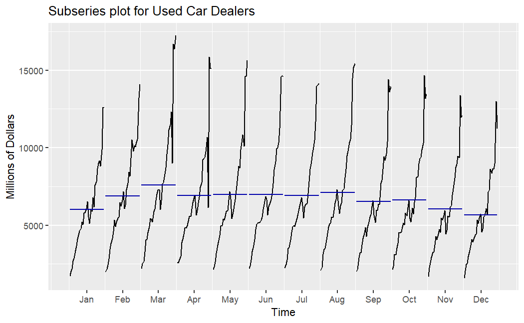
(a) New car (b) Used car

Figure 3: Subseries plot for new car sales(a) and used car sales(b).

To further identify the components contained in the time series, a decomposition of these time series was conducted, and the results are illustrated in Figure 4. It can be noted that these time series demonstrate similar trends. In general, sales gradually increase over time, with slight decreases and fluctuations around 2009 and 2021. Additionally, both time series show seasonality, and the seasonality in the sales of new car is more pronounced, suggesting the potential need for a seasonal ARIMA model.

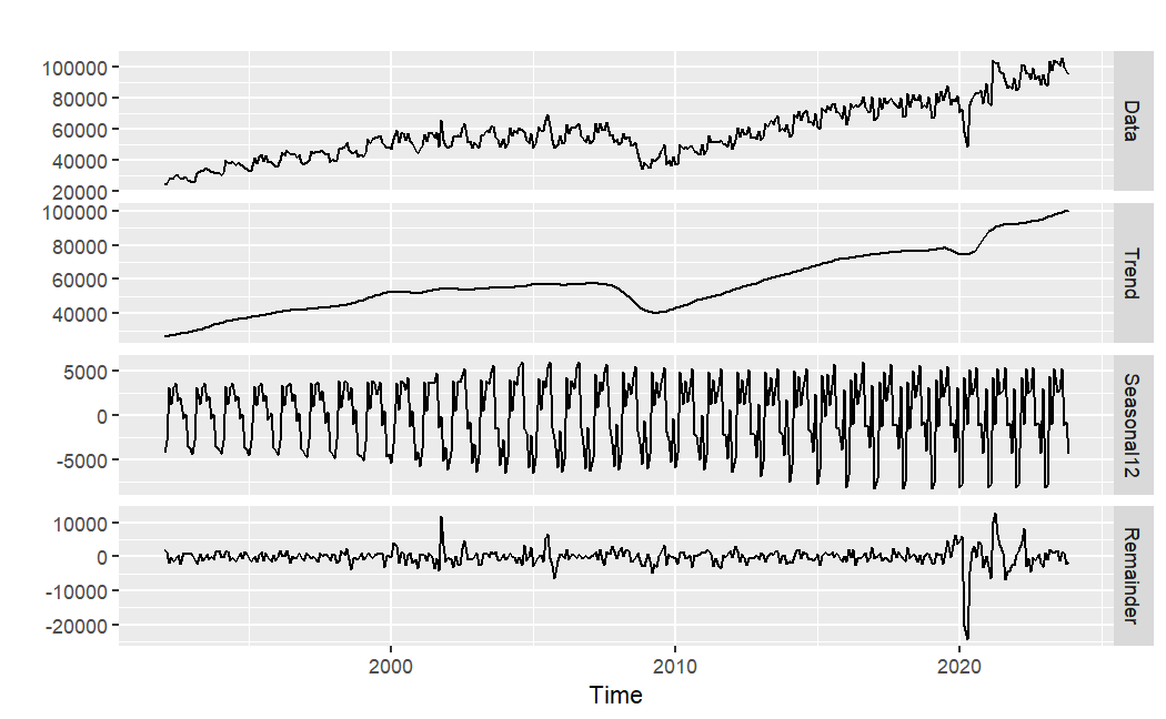
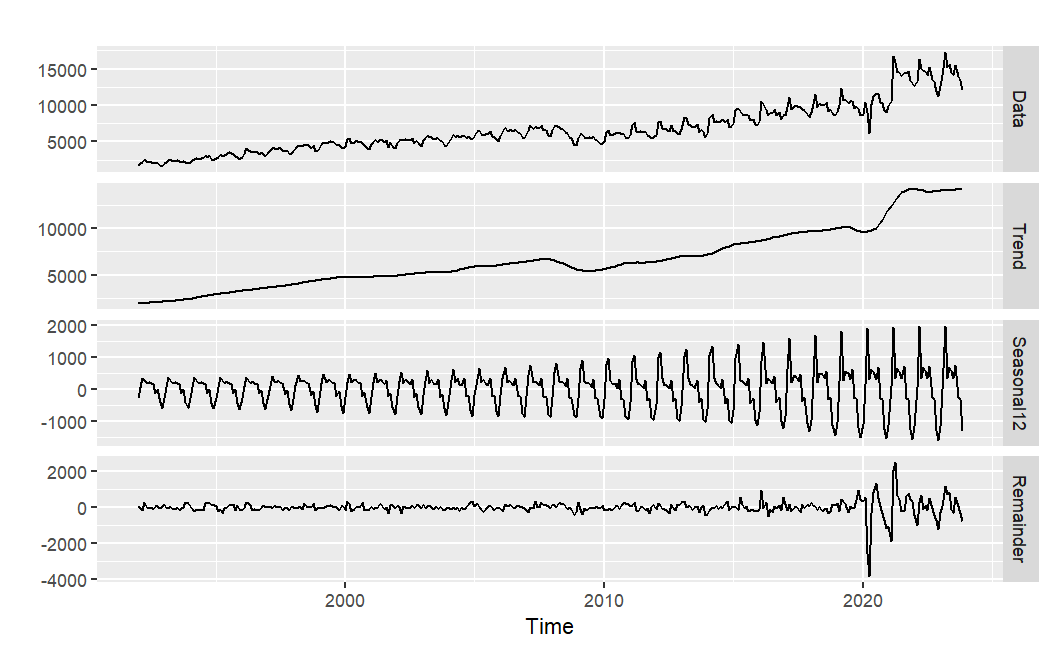
(a) New car (b) Used car

Figure 4: The components of new car sales(a) and used car sales(b).

2.3. Seasonal ARIMA

The ARIMA model necessitates the precondition of data stationarity. Prior to model fitting, the Augmented Dickey-Fuller (ADF) and Kwiatkowski-Phillips-Schmidt-Shin (KPSS) tests are executed to evaluate the stationarity of the time series. The ADF test is based on the assumption that, under the null hypothesis, the data is non-stationary, while it is considered stationary under the alternative hypothesis. In contrast, the KPSS test posits that, under the null hypothesis, the data is stationary, but under the alternative hypothesis, it is non-stationary. The outcomes of the tests are presented in Table 1, revealing that both time series demonstrate non-stationarity based on the p-values.

Table 1: The results of the ADF test and KPSS test (Raw data).

After applying first-order seasonal differencing and logarithmic transformation to the time series, the outcomes of the tests are presented in Table 2, revealing that both time series have become stationary based on the p-values.

Table 2: The results of the ADF test and KPSS test (Processed data).

After applying first-order seasonal differencing and logarithmic transformation to the time series, the time series plots are presented in Figure 5.

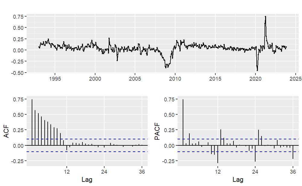
(a) Logarithm transform (b) First-order seasonal difference

Figure 5: Time series plots for data (Logarithm transform and first-order seasonal difference).

Meanwhile, the Partial AutoCorrelation Function (PACF) plots in Figure 5 reveal a strong seasonality in both time series. Therefore, utilizing a Seasonal ARIMA model for fitting would better capture the characteristics of the time series.

The SARIMA model is a powerful instrument in time series analysis for forecasting and modeling. It is an extension of the Autoregressive Integrated Moving Average (ARIMA) model specifically designed to handle time series data with seasonal variations. The SARIMA model's principles encompass four key components: Seasonal Autoregressive, Seasonal Differencing, Seasonal Moving Average, and the three components of the non-seasonal ARIMA model: Autoregressive, Differencing, and Moving Average [11].

Equation (1) can represent the SARIMA (p, d, q) (P, D, Q) ^[m] model:

\( {ϕ_{p}}(B){Φ_{P}}({B^{m}}){(1-B)^{d}}{(1-{B^{m}})^{D}}{y_{t}}={θ_{q}}(B){Θ_{Q}}({B^{m}}){ε_{t}}\ \ \ (1) \)

Where \( p \) denotes the magnitude of non-seasonal AR term, \( P \) denotes the magnitude of seasonal AR term, \( q \) denotes the magnitude of non-seasonal MA term, \( Q \) denotes the magnitude of seasonal MA term, \( d \) represents the magnitude of non-seasonal differencing, \( D \) denotes the magnitude of seasonal differencing, \( m \) denotes the number of observations per year, \( {y_{t}} \) denotes the observed values. \( B \) represents the backshift operator which can be denoted as the following equation 2:

\( {B^{m}}{y_{t}}={y_{t-m}}\ \ \ (2) \)

3. Empirical Results

For new car sales, from the previous analysis, it was determined that due to the non-stationarity of the data and the significant seasonality, first-order seasonal differencing is required. Therefore, it can be preliminarily established that D=1 and d=0. The AutoCorrelation Function (ACF) plot and PACF plot of this time series after logarithmic transformation and first-order seasonal differencing are illustrated in Figure 6. The notable spike at lag 1 in the ACF plot implies the presence of a non-seasonal MA (1) component, while the absence of a significant spike at lag 12 in the ACF plot, and similarly at lag 24, leads to the inference that the magnitude of the seasonal MA component is considered as 0. Meanwhile the notable spike at lag 3 in the PACF plot suggests a non-seasonal AR (3) component, and the notable spike at lag 12 and 24 in the PACF plot indicates the presence of a seasonal AR (2) component.

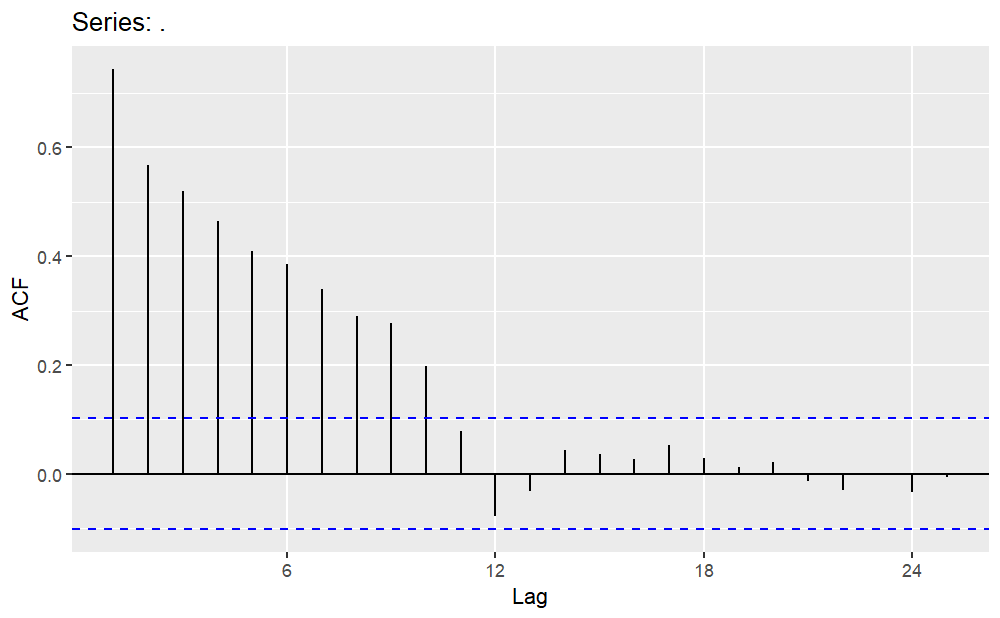
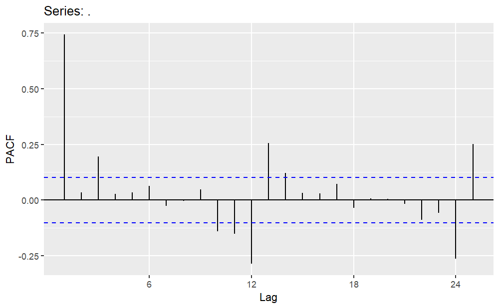
(a) ACF (b) PACF

Figure 6: ACF plot and PACF plot for new car sales (Logarithm transform and first-order seasonal difference).

Therefore, the model is initially set as ARIMA (3, 0, 1) (2, 1, 0) ^[12]. Subsequently, multiple models are fitted, and the fitted models along with their corresponding AICc values, RMSE, MAE, and MAPE are presented in Table 3. By comparing these values, a better-fitting model can be selected. According to the AIC criterion, a superior model has a lower AICc value. Similarly, a model with higher accuracy should have lower errors.

Table 3: Postulated models and corresponding value.

By comparing AICc values, RMSE, MAE, and MAPE, it is observed that the ARIMA (4, 0, 3) (3, 1, 1) ^[12] model is the best-fitting model and also exhibits the highest accuracy. It is noted that, in this case, models with better fit tend to have higher accuracy.

Subsequently, a residual analysis is conducted, and Figure 7 illustrates the results. Furthermore, the Ljung-Box test results in a p-value of 0.2832, implying the acceptance of the null hypothesis and indicating that the residuals show no autocorrelation.

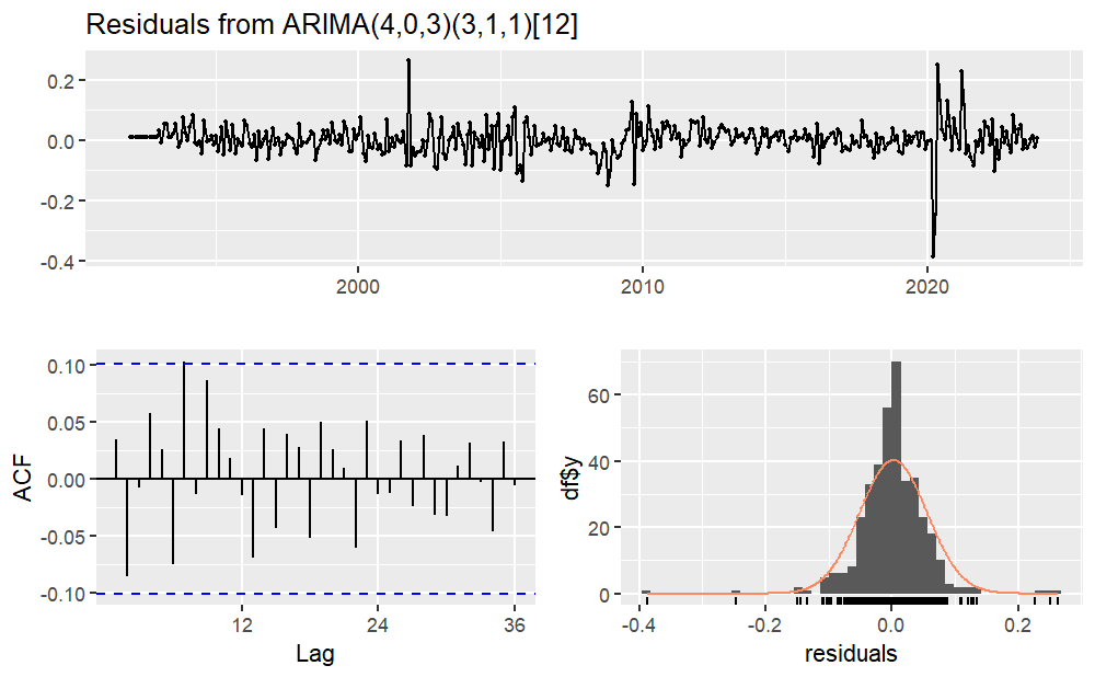
Figure 7: Residuals plot from ARIMA (4,0,3) (3,1,3) ^[12]

Table 4 presents detailed information on the parameters of the ARIMA (4,0,3) (3,1,3) ^[12] model. From the table, it can be observed that, for the sales of new cars, lag periods 1, 2, and 3 exhibit positive autocorrelation with the current period, while lag period 4 shows negative autocorrelation with the current period. Regarding the seasonal lag periods, 1 to 3 exhibit negative autocorrelation with the current period, indicating that an increase in sales in the previous three periods corresponds to a concurrent increase in the current period. From the perspective of seasonal autocorrelation, an increase in sales in the same period of the previous year results in a decrease in the current period's sales.

Analyzing the coefficients of the MA components, the coefficient for MA(1) is significant and positive, indicating that the current observation is positively influenced by past errors. Similarly, the coefficient for SMA(1) is significant and negative, signifying that the current observation is negatively impacted by seasonal errors.

Table 4: Coefficients of ARIMA (4,0,3) (3,1,3) ^[12].

Next, the model is used to forecast the sales volume of new cars for the next two years. As depicted in Figure 8, the forecasted results indicate that sales will continue to exhibit a trend of fluctuating upward growth over the next two years.

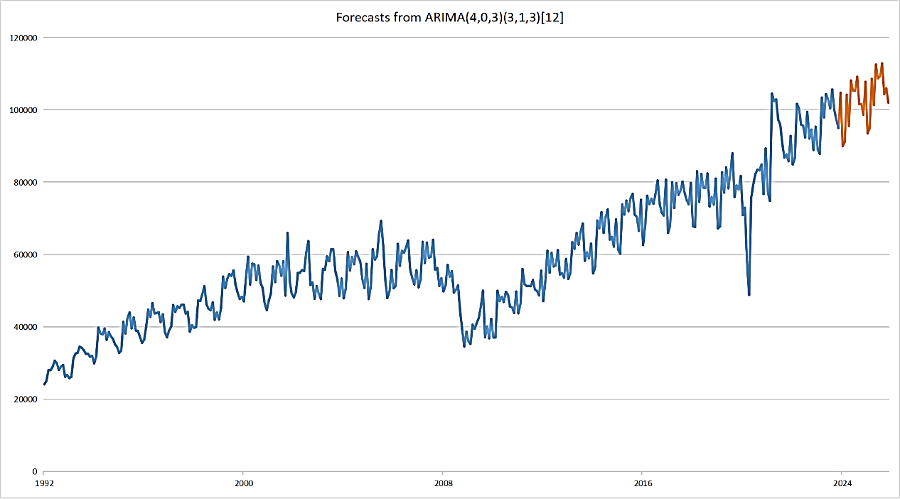
Figure 8: Forecasts from ARIMA (4,0,3) (3,1,3) ^[12]

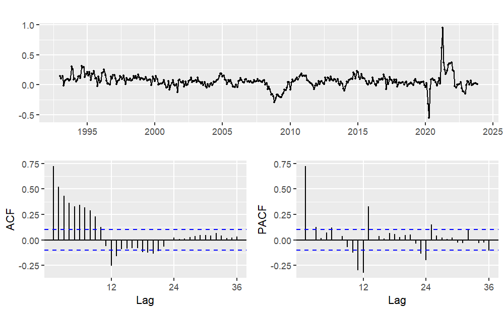
Similarly, for used car sales, from the previous analysis, it was determined that due to the non-stationarity of the time series and the significant seasonality, first-order seasonal differencing is required. Therefore, it can be preliminarily established that D=1 and d=0. The ACF plot and PACF plot of this time series after logarithmic transformation and first-order seasonal differencing are illustrated in Figure 9. The notable spike at lag 1 in the ACF plot implies the presence of a non-seasonal MA (1) component, while the notable spike at lag 12 in the ACF plot leads to the inference that the magnitude of the seasonal MA component is considered as 1. Meanwhile the notable spike at lag 2 in the PACF plot implies the presence of a non-seasonal AR (2) component, and the notable spike at lag 12 and 24 in the PACF plot indicates the presence of a seasonal AR (2) component.

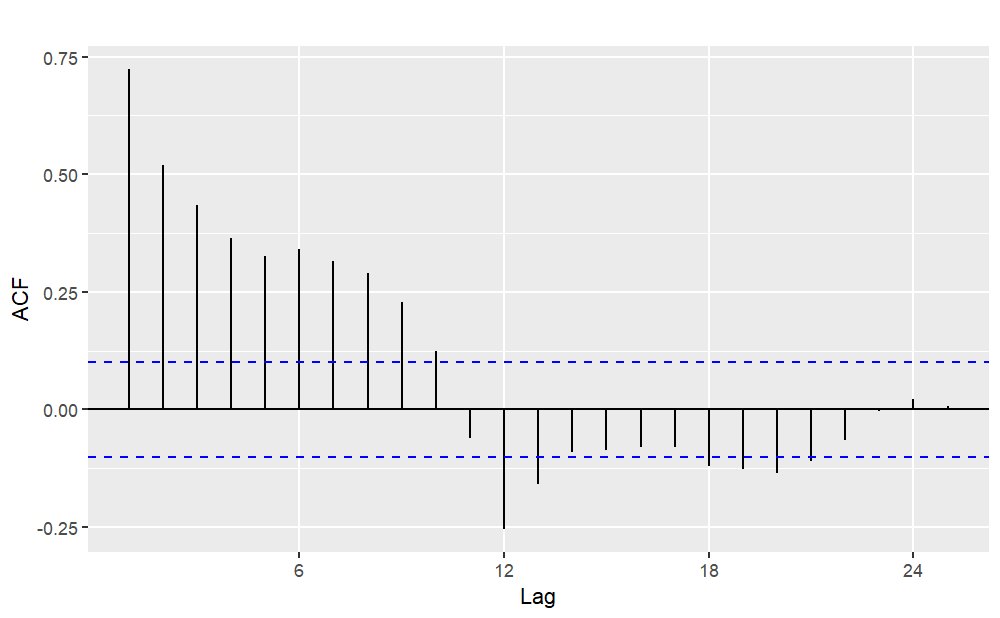
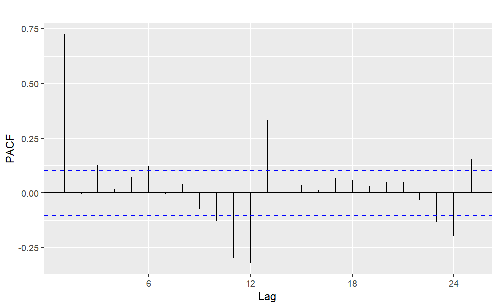
(a) ACF (b) PACF

Figure 9: ACF plot and PACF plot for used car sales (Logarithm transform and first-order seasonal difference).

Therefore, the model is initially set as ARIMA (2, 0, 1) (2, 1, 1) ^[12]. Subsequently, multiple models are fitted, and the fitted models along with their corresponding AICc values, RMSE, MAE, and MAPE are presented in Table 5. Continue to identify a better-fitting model by comparing these values.

Table 5: Postulated models and corresponding value.

By comparing AICc values, it was found that ARIMA (2, 0, 1) (2, 1, 1) ^[12] is the best-fitting model among these models. However, the ARIMA (2, 0, 3) (2, 1, 3) ^[12] model has the lowest RMSE, MAE, and MAPE. In the pursuit of higher forecast accuracy, the final choice is to use the ARIMA (2, 0, 3) (2, 1, 3) ^[12] model for forecasting the used car sales. It is noted that, in this case, models with better fit tend to have higher accuracy.

Subsequently, a residual analysis is conducted, and Figure 10 illustrates the results. Furthermore, the Ljung-Box test results in a p-value of 0.2039, implying the acceptance of the null hypothesis and indicating that the residuals show no autocorrelation.

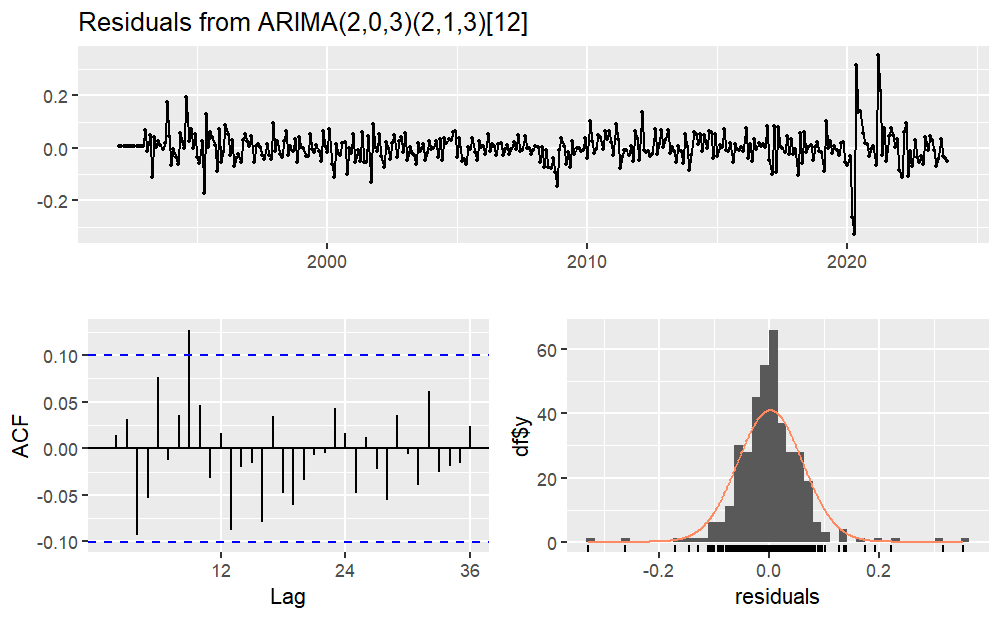
Figure 10: Residuals plot of ARIMA (2,0,3) (2,1,3) ^[12]

Table 6 displays detailed information about the parameters of the ARIMA (2,0,3) (2,1,3) ^[12] model. From the table, it is evident that, for the sales of used cars, lag period 2 exhibits a significant positive autocorrelation with the current period. Regarding the seasonal lag period, the coefficient for SAR(1) is significant and negative, indicating that an increase in sales in lag period 2 corresponds to a concurrent increase in the current period. From the perspective of seasonal autocorrelation, an increase in sales in the same period of the previous year results in a decrease in the current period's sales.

Analyzing the coefficients of the MA components, the coefficient for MA(1) is significant and positive, signifying that the current observation is positively influenced by past errors. Similarly, the coefficients for MA(2) and MA(3) are significant and negative, indicating that the current observation is negatively impacted by past errors. Likewise, the coefficient for SMA(2) is significant and negative, suggesting that the current observation is negatively influenced by seasonal errors.

Table 6: Coefficients of ARIMA (2,0,3) (2,1,3) ^[12].

Next, the model is used to forecast the sales volume of used car for the next two years. As depicted in Figure 11, the forecasted results indicate that sales will continue to exhibit a trend of fluctuating upward growth over the next two years.

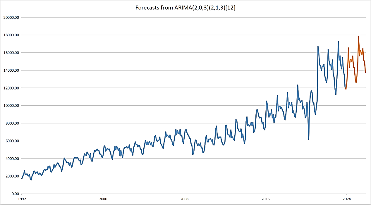
Figure 11: Forecasts from ARIMA (2,0,3) (2,1,3) ^[12]

4. Conclusion

In conclusion, this paper of new and used car sales time series in the United States using SARIMA models has yielded valuable insights into the overall trends and seasonality of the market. While the selected models, ARIMA (4, 0, 3) (3, 1, 1) ^[12] for new car sales and ARIMA (2, 0, 3) (2, 1, 3) ^[12] for used car sales, have demonstrated efficacy in capturing time series characteristics and forecasting, there are notable considerations and opportunities for improvement.

The coefficients of the model also reveal that, for new car sales, the presence of positive autocorrelation in lag periods 1, 2, and 3, along with negative seasonal autocorrelation in lag period 1, suggests that an increase in sales in the previous three periods will lead to a corresponding increase in the current period's sales. From the perspective of seasonal autocorrelation, however, an increase in sales in the same period of the previous year will result in a decrease in the current period's sales. Furthermore, the current period's sales are positively influenced by past errors and negatively impacted by seasonal errors.

On the other hand, for used car sales, the existence of positive autocorrelation in lag period 2 and negative seasonal autocorrelation in lag period 1 indicates that an increase in sales in lag period 2 will correspondingly increase the current period's sales. From the perspective of seasonal autocorrelation, an increase in sales in the same period of the previous year will lead to a decrease in the current period's sales. Additionally, the current period's sales are influenced positively by MA(1) and negatively by MA(2) and MA(3), along with negative impacts from seasonal errors.

The practical implications of this paper extend to both sellers and buyers in the automotive industry, providing a basis for strategic decision-making. However, it is essential to acknowledge the limitations of our study, including the reliance on a specific model type and the exclusion of certain influencing factors. Future research endeavors could explore incorporating additional models such as VAR or GARCH, offering a more comprehensive understanding of market dynamics.

The challenges in model selection, particularly the discrepancy between AICc values and forecast errors in used car sales, highlight the intricacies of forecasting in dynamic markets. Exploring the reasons behind this divergence and refining the model selection process will be crucial for advancing forecast accuracy.

While the forecasts indicate sustained upward-trending fluctuations in sales volumes over the next two years, it is worth noting the importance of considering external factors that could influence these trends. Decision-makers should approach these forecasts with an awareness of the ever-changing landscape and be prepared to adapt strategies accordingly.

In recommending further avenues for research, it is worth noting the exploration of alternative models and methods, such as artificial neural networks, to enhance forecast accuracy and uncover additional nuances within the time series. The iterative nature of forecasting underscores the need for continuous improvement and adaptation to evolving market conditions, reinforcing the dynamic relevance of our research in the automotive industry.

References

[1]. Kohli, S., Godwin, G. T., & Urolagin, S. (2020). Sales prediction using linear and KNN regression. In Advances in Machine Learning and Computational Intelligence: Proceedings of ICMLCI 2019 (pp. 321-329): Springer.
[2]. Fantazzini, D., & Toktamysova, Z. (2015). Forecasting German car sales using Google data and multivariate models. International Journal of Production Economics, 170, 97-135.
[3]. Wenshun, Sheng., Hanchi, Zhao., & Yanwen, Sun. (2019). Sales Forecasting Model Based on Improved Genetic Algorithm Optimized BP Neural Network. Computer Systems & Applications, 28(12), 200-204.
[4]. Permatasari, C. I., Sutopo, W., & Hisjam, M. (2018). Sales forecasting newspaper with ARIMA: A case study. Paper presented at the AIP Conference Proceedings.
[5]. Pavlyshenko, B. M. (2019). Machine-learning models for sales time series forecasting. Data, 4(1), 15.
[6]. Jingli, Guo., & Bo, Dong. (2019). International Rice Price Forecast Based on SARIMA Model. Price Theory and Practice, 01, 79-82.
[7]. Zhilin, Chen., Hongtao, Hu., & Yingying, Bian. (2024). Forecasting Shanghai Port Container Throughput under the COVID-19 Pandemic Using the SARIMA Model. Industrial Engineering and Management, 01, 32-40.
[8]. Farhan, J., & Ong, G. P. (2018). Forecasting seasonal container throughput at international ports using SARIMA models. Maritime Economics & Logistics, 20, 131-148.
[9]. Hao, Huang., & Yingmei, Deng. (2023). Forecast Analysis of Neurosurgical Workload in a Tertiary Hospital Based on the SARIMA Model. Chinese Medical Records, 11, 52-54.
[10]. Wanning, Sun., Jing, Yang., & Yiyi, Yang. (2018). Analysis and Forecast of China's GDP Based on SARIMA Model. Chinese Collective Economy, 36, 78-80.
[11]. Shumway, R. H., Stoffer, D. S., & Stoffer, D. S. (2000). Time series analysis and its applications (Vol. 3). New york: Springer.
Cite this article
Chen,J. (2024). Time Series Analysis and Forecast of Sales of New Car and Used Car Using SARIMA Model. Advances in Economics, Management and Political Sciences,86,122-132.
Data availability
The datasets used and/or analyzed during the current study will be available from the authors upon reasonable request.
Disclaimer/Publisher's Note
The statements, opinions and data contained in all publications are solely those of the individual author(s) and contributor(s) and not of EWA Publishing and/or the editor(s). EWA Publishing and/or the editor(s) disclaim responsibility for any injury to people or property resulting from any ideas, methods, instructions or products referred to in the content.
About volume
Volume title: Proceedings of the 2nd International Conference on Management Research and Economic Development
© 2024 by the author(s). Licensee EWA Publishing, Oxford, UK. This article is an open access article distributed under the terms and
conditions of the Creative Commons Attribution (CC BY) license. Authors who
publish this series agree to the following terms:
1. Authors retain copyright and grant the series right of first publication with the work simultaneously licensed under a Creative Commons
Attribution License that allows others to share the work with an acknowledgment of the work's authorship and initial publication in this
series.
2. Authors are able to enter into separate, additional contractual arrangements for the non-exclusive distribution of the series's published
version of the work (e.g., post it to an institutional repository or publish it in a book), with an acknowledgment of its initial
publication in this series.
3. Authors are permitted and encouraged to post their work online (e.g., in institutional repositories or on their website) prior to and
during the submission process, as it can lead to productive exchanges, as well as earlier and greater citation of published work (See
Open access policy for details).