1. Introduction

There is no absolute fairness in the world. Problems regarding fairness arise every day, and humanity is continually on the course of seeking relative fairness. Fairness issues are involved in the majority of social processes, among which is the distribution fairness that is discussed in this paper.

The problem will be solved and discussed is set in this background: By the beginning of the 23rd century, mankind has settled Mars, the Moon and other bodies of the solar system. Under the direction of a heuristically programmed algorithmic computer HAL-13, the Humankind Post Global System is delivering cargoes between numerous colonies and space stations. IMMC team, Alice, Bob, Charlie, David and Erin live on a remote research base on Mars. One fine day, a transport Humankind Post ship arrives at the base with cargo that was clearly destined for some other addressees. But HAL-13 denies the error, denies the arrival of the transport and the very existence of this ship. Since it is impossible to return the shipment, the researchers decide to split the goods among themselves.

In this paper, we first define what is fairness, and then create a model to determine the optimal assignment option corresponding to each definition of fairness which is transferred into formulas and established via the models. Finally, data is applied in Zero-one integer programming, testing the model in the context of a realistic problem.

Also, refinements are made to improve the model so that it’ll be more applicable and practical. We include social interactions, competition, and collaboration, into consideration with a new set of calculations provided in this context. We also determine the possession and combination of different items influence one’s valuation of the product. Finally, we use the model that we have refined after the calculations of different scenarios to find what will the allocation of items be for 5 researchers.

2. Preliminary Assumptions and Definitions

2.1. Assumptions

Assumption 1: Fairness is relative therefore can be clearly defined. This assumption is the basis of our definition of fairness because what is fairness is a philosophical problem and hard to define, we assume that fairness can be defined and thus be expressed in the form of a formula. Accordingly, we can transfer fairness into limitations and put them in the model.

Assumption 2: Fairness can be determined via purely quantitative means. This assumption is the basis of our definition of fairness. Additionally, there are already many diverse quantitative measures available to employ in modeling, so limiting the factors used to quantitative ones will still provide a comprehensive result.

Assumption 3: Each person's valuation is aligned with their thoughts and their valuation is transparent without any information hidden deliberately. For the sake of simplicity and straightforwardness, we assume that each person gives their valid subjective valuation independently.

Assumption 4: Each item is unique and cannot be further divided. Dividing the items in the list to several persons may destroy items thus lowering the subjective valuations given by each person, and provided that some items cannot be divided, making sure that each item can only be given to one person can ensure the authenticity and credibility of the result produced by the model.

Assumption 5: The value of a thing can and can only be measured by valuation. To make the results only based on each person’s valuations, we assume that other factors like market price have no influence on the valuation of items.

2.2. Variable Chart

Table 1: Variable Definitions

3. Related works of definition of Fairness and Assessment

3.1. Fairness Definition

As said in the Introduction, there’s no absolute fairness. Therefore, different definitions of fairness may end in different allocation scenarios. Taking social, philosophical, and market factors into consideration, the following definitions of fairness are listed below:

Define by Utilitarianism

From a utilitarian perspective, fairness is achieved when resource distribution maximizes overall societal happiness or well-being [1]. In this context, the happiness of attaining an item for these five people is reflected in their evaluations, where a higher evaluation by a certain person indicates a higher happiness [2]. Therefore, achieving maximized fairness, under the utilitarian view, means distributing items according to each person’s preference [3]. Whoever evaluates an item with the highest price will derive the item.

Defined by Definite Amount Equality

To distribute items merely considering their amount, disregarding the value of each item, and treating them as if they are identical, is a reasonable perspective of equality. In this situation, specifically, 30 items are allocated to 5 people, thus receiving 6 items for each person.

Defined by Veil of Ignorance (VI)

This is the distribution scheme corresponding with the philosophical assumption, Vein of Ignorance. Suppose one of the five people is required to dictate the scheme of allocating but is ignorant of whom he or she will be, the allocation dictated should favor the disadvantaged groups, in this case, to maximize the least sum of total value of individual researchers [4].

Combining Amount Equality and Veil of Ignorance

Distributing by pure amount equality and by pure Veil of Ignorance is both defective. The former lacks the confine of value, which may end in some researchers getting more inferior items while others getting more superior items. The latter, on the other hand, overlooks the quantity, which may result in some getting a lot of inferiors while others getting few superiors.

Defined by Markets with Equal Initial Budgets for Each Researcher

In this situation, allocation from fair market competition is considered fair. Each researcher receives a same initial budget, and they cost their budgets when receiving an item with the price of their evaluation [5]. In other words, the evaluation of every item is how much the researcher can accept paying.

3.2. Fairness Assessment

Quantitatively measuring fairness is imperative for assessing the fairness of an allocation, once each definition is clearly defined. The ensuing definitions will translate abstract notions of fairness into specific and measurable expressions [6].

3.2.1. Fairness Deviation

The fairness deviation, denoted as σ, is defined to quantify the extent to which an allocation deviates from the optimal allocation according to a specific fairness definition. Consequently, σ varies across different definitions.

• Pure amount: Under the pure amount definition, its fairness deviation, \( {σ_{1}} \) , is defined as:

\( {σ_{1}}=\frac{S}{3n} \) (1)

• Veil of Ignorance: Under the pure value definition, its fairness deviation, \( {σ_{2}} \) , is defined as:

\( {σ_{2}}=\frac{{∑_{i}}{∑_{j}}{x_{i,j}}×{P_{i,j}}}{3n} \) (2)

• Amount equality and the Veil of Ignorance: Combining the pure value definition and pure amount definition, its fairness deviation, \( {σ_{3}} \) , is defined as:

\( {σ_{3}}={e^{{σ_{1}}+\frac{{σ_{2}}}{100}}} \) (3)

e-exponent is used here to ensure when \( {σ_{i}}=0 \) the equation will not equal 0 directly. This is the same reason for the definition of \( {φ_{3}} \) .

• Utilitarianism: Under the Utilitarianism definition, its fairness deviation, \( {σ_{4}} \) , is defined as:

\( {σ_{4}}=\frac{max{\lbrace ∑_{i}}{∑_{j}}{x_{i,j}}×{P_{i,j}}\rbrace -min{\lbrace ∑_{i}}{∑_{j}}{x_{i,j}}×{P_{i,j}}\rbrace }{3} \) (4)

3.2.2. Fairness Coefficient

Define the optimal coefficient, \( {φ_{1}} \) , for pure amount equality as

\( {φ_{1}} =\frac{{∑_{i}}(|{∑_{i}}{x_{i,j}}-\frac{S}{n}|)}{n} \) (5)

Define the optimal coefficient, \( {φ_{2}} \) , for the Veil of Ignorance as

\( {φ_{2}}=\frac{max⁡\lbrace {∑_{i}}{x_{i,j}}×{P_{i,j}}\rbrace -min{\lbrace ∑_{i}}{x_{i,j}}×{P_{i,j}}\rbrace }{2} \) (6)

Define the optimal coefficient, \( {φ_{3}} \) , for the combination of amount equality and the Veil of Ignorance as

\( {φ_{3}}={e^{{φ_{1}}+\frac{{φ_{2}}}{100}}} \) (7)

Define the optimal coefficient, \( {φ_{4}} \) , for Utilitarianism as

\( {φ_{4}}=max{\lbrace ∑_{i}}{∑_{j}}{x_{i,j}}×{P_{i,j}}\rbrace -{∑_{i}}{∑_{j}}{x_{i,j}}×{P_{i,j}} \) (8)

3.2.3. Fairness Extent

\( φ \) will be compared with \( σ \) to determine fairness extension:

• If \( {φ_{i}} \lt {σ_{i}} \) , then its deviation has a relatively small value. In this case, the allocation will be called fair for this definition.

• If \( {σ_{i}} \) < \( {φ_{i}} \lt 2{σ_{i}} \) , then its deviation has a medium value. In this case, the allocation will be called relatively fair for this definition.

• If \( {φ_{i}} \gt 2{σ_{i}} \) , then its deviation has a large value. In this case, the allocation will be called unfair for this definition.

For the third definition, the criterion is a little different since it involves an e-exponent. Napierian logarithm is used to derive a comparable result:

\( α=ln⁡(\frac{{φ_{3}}}{{σ_{3}}}) \) (9)

• If \( α \lt 0 \) , the allocation will be called fair for this definition.

• If \( 0 \lt α \lt 5 \) , the allocation will be called relatively fair for this definition.

• If \( α \gt 5 \) , the allocation will be called unfair for this definition.

4. Modelling

4.1. Zero-one Integer Programing

In the model, zero-one integer programming is used to incorporate criteria that can be modelled linearly [7]. These criteria can be either objective functions to be maximized or minimized, or restrictions on those functions. The variables involved are assumed to be continuous. The resulting solution is definitive and represents the best possible solution, given the available resources and restrictions imposed.

4.2. Criteria 1: Allocation Under Utilitarianism

Under utilitarianism, the society aims to maximize the overall welfare, by allocating an item to the person who value it most. The allocation option that yields the highest results should be the “best” in that aspect, as it would have the highest fairness, provide the item to researchers who prefers it most. Similar to the model in Section 3, this criterion extends the allocation from 2 researchers to 5.

max \( {∑_{i}}{∑_{j}}{x_{i,j}}×{P_{i,j}} \) (10)

s.t. \( \sum _{j}{x_{i,j}}=1 \) (11)

Where P is the overall value, \( {x_{i,j}} \) is the possession of item i for person j, \( {P_{i,j}} \) is the value of item i evaluated by person j.

4.3. Criteria 2: Allocation Under Equality by Number of Items

On the base of maximizing total values, the number of items every researcher get should be same, which is 6 in this situation.

max \( {∑_{i}}{∑_{j}}{x_{i,j}}×{P_{i,j}} \) (12)

s.t. \( \begin{cases} \begin{array}{c} {∑_{i}}{x_{i,j}}=6 \\ \sum _{j}{x_{i,j}}=1 \end{array} \end{cases} \) (13)

Where P is the overall value, \( {x_{i,j}} \) is the possession of item i for person j, \( {P_{i,j}} \) is the value of item i evaluated by person j.

4.4. Criteria 3: Allocation Under Veil of Ignorance

According to Rawls’ Veil of Ignorance, people would have to prepare for the disadvantage situation and prefer an allocation of resources to lift the living standards of the lower class. Translating to our model, the society aims to maximize the total value that is possessed by the researcher who are allocated with lowest value of items, a max-min model was used to maximize the least sum of total value of individual researchers.

max Z(14)

s.t. \( j \) 𝑥𝑖,𝑗=1𝑖𝑥𝑖,𝑗×𝑃𝑖,𝑗≥𝑍 s.t. \( \begin{cases} \begin{array}{c} \sum _{j}{x_{i,j}}=1 \\ \sum _{i}{x_{i,j}}×{P_{i,j}}≥Z \end{array} \end{cases} \) (15)

Where P is the overall value, \( {x_{i,j}} \) is the possession of item i for person j, \( {P_{i,j}} \) is the value of item i evaluated by person j, Z is an auxiliary variable that denotes the minimum individual sum of value.

4.5. Criteria 4: Allocation Definite Amount Equality and Under VI

Since allocation merely under definite amount equality results in significant differences in individual value, and allocation under Veil of Ignorance causes discrepancy in number of items, this model combines the two criteria and fully take advantage of each criteria’s properties.

max Z(16)

s.t. \( \begin{cases} \begin{array}{c} \sum _{j}{x_{i,j}}=1 \\ \sum _{i}{x_{i,j}}×{P_{i,j}}≥Z \\ {∑_{i}}{x_{i,j}}=6 \end{array} \end{cases} \) (17)

Where P is the overall value, \( {x_{i,j}} \) is the possession of item i for person j, \( {P_{i,j}} \) is the value of item i evaluated by person j, Z is an auxiliary variable that denotes the minimum individual sum of value.

4.6. Criteria 5: Allocation Under Markets with Equal Initial Budgets

This model represents the allocation under markets, where every researcher receives items by costing their evaluations on it, and the total cost cannot exceed the same initial budget for everyone.

max \( {∑_{i}}{∑_{j}}{x_{i,j}}×{P_{i,j}} \) (18)

\( s.t.\begin{cases} \begin{array}{c} \sum _{j}{x_{i,j}}=1 \\ \sum _{i}{x_{i,j}}×{P_{i,j}}≤B \end{array} \end{cases} \) (19)

Where P is the overall value, \( {x_{i,j}} \) is the possession of item i for person j, \( {P_{i,j}} \) is the value of item i evaluated by person j, B is the initial budget.

4.7. Model’s Refinement

In this section, the model is refined by considering social interaction between researchers. Two models are established according to different situations: relationship and auction.

4.7.1. Situation 1: Allocation with Relationship Matrix

In this model, three types of relationships are defined:

• Collaboration means the researchers having this relationship will share their gains, benefiting each other. The quantitative description is once one of the collaborators gets an item, all the researchers who collaborate with him will be added 0.2 \( { P_{i,j}} \) to their total value where \( { P_{i,j}} \) refers to the value of the item i the researcher j gets.

• Competition means the researchers having this relationship will bring bad effects when either one of them receives an item, harming the others. The quantitative description is once one of the competitors gets an item, all the researchers who compete with him will be subtracted 0.2 \( { P_{i,j}} \) from their total value.

• No Relation means there is no relationship between the researchers having this relationship. One of them gaining an item will not affect others, thus maintaining each of their total values the same.

Therefore, their mutual relationships can be expressed in a symmetric matrix. Since the problem provide no relationship between these researchers, the following relationship is randomly generated for the researchers as an example:

\( [\begin{matrix}1 & 0.2 & -0.2 & 0 & 0 \\ 0.2 & 1 & 0 & 0 & -0.2 \\ -0.2 & 0 & 1 & 0.2 & 0 \\ 0 & 0 & 0.2 & 1 & -0.2 \\ 0 & -0.2 & 0 & -0.2 & 1 \\ \end{matrix}] \) (20)

Relationship Matrix (0.2 Ally, -0.2 Rival, Neutral 0, 1 self)

Incorporating this matrix, the following model is derived:

max \( \sum _{i}\sum _{j}\sum _{k}{x_{i,j}}×{P_{i,j}}×{R_{j,k}} \) (21)

s.t. \( \sum _{j}{x_{i,j}}=1 \) (22)

Where P is the overall value, \( {x_{i,j}} \) is the possession of item i for person j, \( {P_{i,j}} \) is the value of item i evaluated by person j, \( {R_{j,k}} \) is the relationship between j and k

4.7.2. Situation 2: Allocation by Auction

In this model, each researcher is given a certain budget initially and they will conduct an auction process, where each researcher increases their bidding price until the bidding price exceeds their subjective value or no one else competes. Therefore, the bidding price stops at the second highest value plus one, which is defined as \( {M_{i}} \) . The researcher who wins the item enjoys the consumer surplus \( {(P_{i,j}}-{M_{i}}) \) . The objective for this society is to maximize the total consumer surplus.

max \( \sum _{i}\sum _{j}{x_{i,j}}×{(P_{i,j}}-{M_{i}}) \) (23)

\( s.t.\begin{cases} \begin{array}{c} \sum _{j}{x_{i,j}}=1 \\ \sum _{i}{x_{i,j}}×{M_{i}}≤B \end{array} \end{cases} \) (24)

Where P is the overall value, \( {x_{i,j}} \) is the possession of item i for person j, \( {P_{i,j}} \) is the value of item i evaluated by person j, B is the initial budget, \( {M_{i}} \) is the market price or bidding price for item i.

4.7.3. Situation 3: Allocation with Complement and Substitute Gains

Researchers’ subjective value of goods may change depending on the possession situation of cargoes. To quantify the distinction of judgment, a gain matrix is adopted in our mathematics model through our thorough discussion of different relationships within different cargoes [8].

Gain Matrix

In the following is an example from our gain matrix that pairs different items together and finds whether some pairs got by one person would increase, or decrease their total value by considering complements and substitutes. Otherwise, the total value of the pairs would stay the same.

Complement and substitute are divided into 5 levels: Complements: 0.2, Relative Complementary: 0.1, No relationship: 0, relative substitutional: -0.1, Substitutes: -0.2

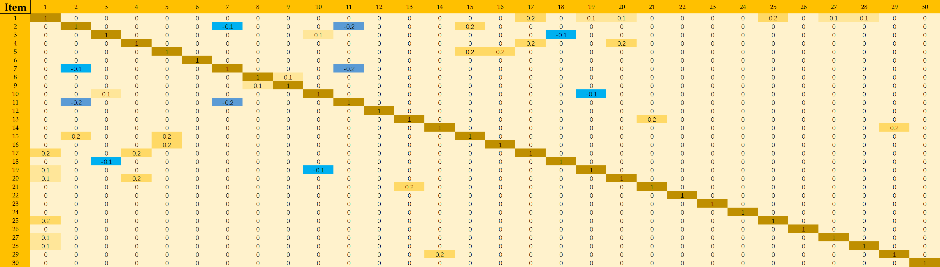
Figure 1: Gain Matrix

When the subjective value of researchers can be influenced by different possession situations of others, it is necessary to introduce new variables into the original zero-one integer programming model. These variables include \( {G_{i,k}} \) , which represents the gaining coefficient from the Gain Matrix, and \( {x_{k,j}} \) , indicating whether researcher j possesses item k. Building upon the previously defined model and incorporating the new situation, the updated model becomes:

max \( \sum _{i}\sum _{j}\sum _{k}{G_{i,k}}×{x_{k,j}}×{x_{i,j}}×{P_{i,j}} \) (25)

s.t. \( \sum _{j}{x_{i,j}}=1 \) (26)

5. Applications

In this section, the models designed are applied respectively to find the different distribution results of cargoes and comparing them.

5.1. Result for Criteria 1: Allocation Under Utilitarianism

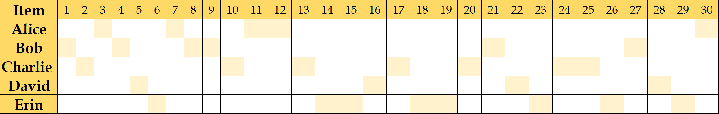
Figure 2: Allocation Result for Task 2.1

The accurate numbers and values for each member listed as Alice for 5 items and 166 acr, Bob for 6 items and 985.0 acr, Charlie for 7 items and 1100.0 acr, David for 4 items and 1610.0 acr, Erin for 8 items and 1215.0 acr.

5.2. Result for Criteria 2: Allocation Under Equality by Number of Items

Figure 3: Allocation Result for Task 2.2

Besides five items for every members, the accurate values for each member listed as Alice for 186.0 acr, Bob for 985.0 acr, Charlie for 1075.0 acr, David for 1633.0 acr, Erin for 1180.0 acr.

5.3. Result for Criteria 3: Allocation Under Veil of Ignorance

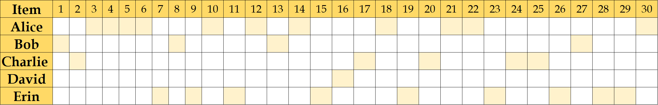
Figure 4: Allocation Result for Task 2.3

The accurate values for each member listed as Alice for 11 items and 900.0 acr, Bob for 4 items and 910.0 acr, Charlie for 5 items and 900.0 acr, David for 1 items and 1100.0 acr, Erin for 9 items and 900.0 acr.

5.4. Result for Criteria 4: Allocation Definite Amount Equality and Under VI

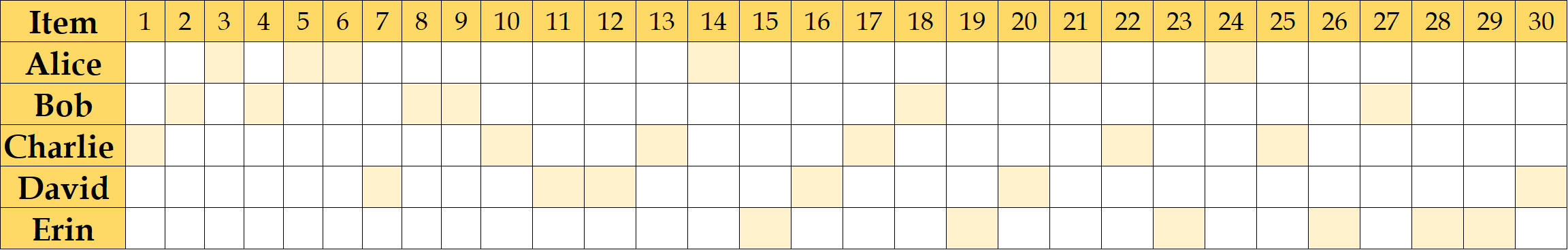
Figure 5: Allocation Result for Task 2.4

Besides the 6 items for each member, the accurate values for each member listed as Alice for 860.0 acr, Bob for 882.0 acr, Charlie for 875.0 acr, David for 1138.0 acr, Erin for 890.0 acr.

5.5. Result for Criteria 5: Allocation Under Markets with Equal Initial Budgets

5.5.1. Result under B = 1500

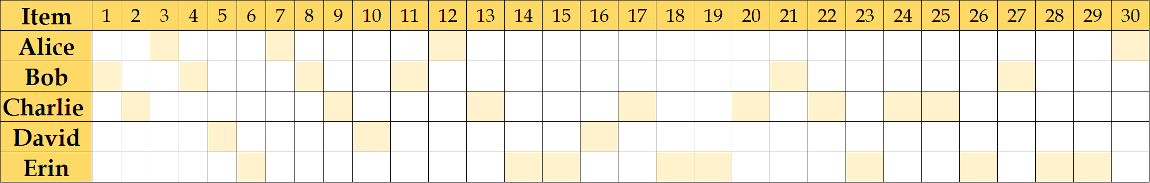
Figure 6: Allocation Result for Task 2.5

Under 1500 acr budget, the accurate numbers and values for each member listed, as Alice for 4 items and 162 acr, Bob for 7 items and 989 acr, Charlie for 8 items and 1195 acr, David for 3 items and 1490 acr, Erin for 8 items and 1235acr.

5.5.2. Sensitivity Analysis

Budget can be tested and manipulated to conduct a sensitivity analysis of zero-one integer programming. The budget is adjusted from 500 to 2000 with a unit increment of 100, resulting in the change of total value and total numbers of items. Figure 11 indicates the fluctuation in stacked graphs.

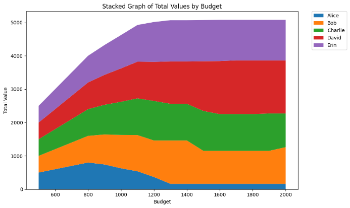
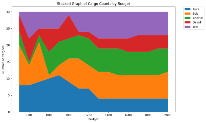
Figure 7: Stacked Graphs of Total Values and Numbers

The sensitivity analysis graph for total values shows an increase of values from 500 to 1200, suggesting that as budget increases, each researcher are able to receive objects with higher values. From 1200 to 2000, the fluctuation mitigates, indicating that the budget has less effect on the allocation results.

The sensitivity analysis graph for total numbers shows an irregularly fluctuation of numbers from 500 to 1200, suggesting that the number of items each researcher got is restricted by the tight budget. From 1200 to 2000, the fluctuation mitigates, indicating that the budget no longer becomes the restriction.

5.6. Results under Social Interactions

5.6.1. Result for Situation 1: Allocation with Relationship Matrix

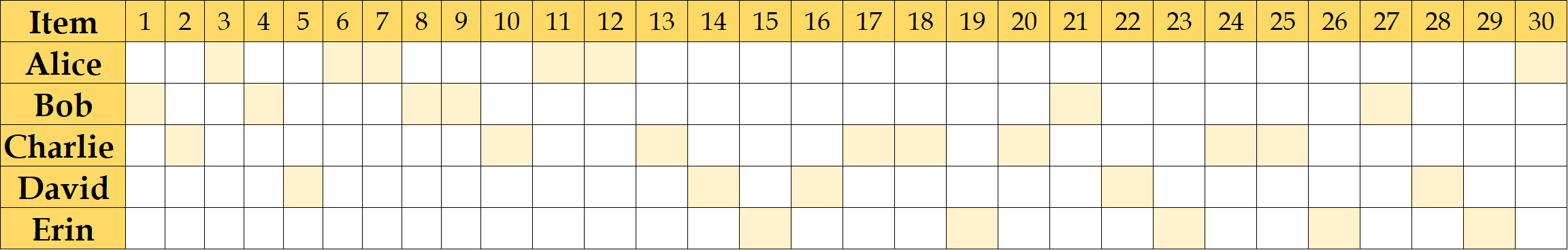
Figure 8: Allocation Result for Task 3.1

The accurate values for each member listed as Alice for 6 items and 346.0 acr, Bob for 6 items and 985.0 acr, Charlie for 8 items and 1120.0 acr, David for 5 items and 1740.0 acr, Erin for 5 items and 845.0 acr.

5.6.2. Result under Situation 2: Allocation by Auction

Results under B = 1500:

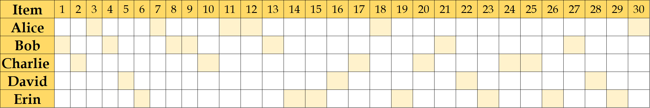
Figure 9: Allocation Result for Task 3.2

Under 1500 acr budget, the accurate numbers for each member listed, as Alice for 6 items and 186 acr, Bob for 7 items and 1095 acr, Charlie for 6 items and 990 acr, David for 4 items and 1590 acr, and Erin for 7 items and 1215 acr.

Sensitivity Analysis:

Budget can be tested and manipulated to conduct a sensitivity analysis of zero-one integer programming. The budget is adjusted from 100 to 2000 with a unit increment of 100, resulting in the change of total value and total numbers of items. Figure 14 indicates the fluctuation in stacked graphs.

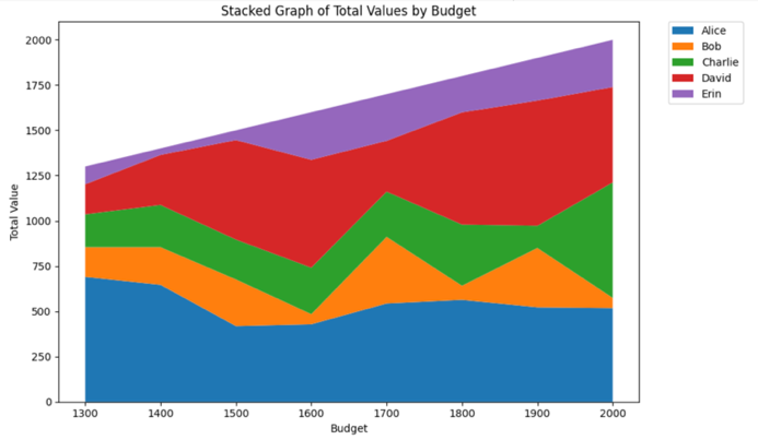
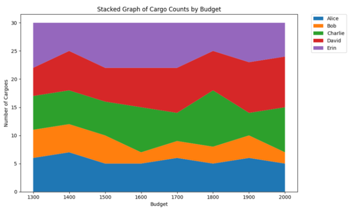
Figure 10: Stacked Graphs of Total Values and Numbers

The sensitivity analysis graph for total values shows an increase of values from 1300 to 2000, suggesting that as budget increases, the overall value among five researchers increases, but individual total value remains relatively constant, indicating that the budget is a restrain to overall values not individual values.

The sensitivity analysis graph for total numbers shows a relatively low fluctuation of numbers from 1300 to 2000, suggesting that the budget is not the restriction to number of items.

5.6.3. Result under Situation 3: Allocation with Complement and Substitute Gains

Figure 11: Allocation Result for Task 4

The accurate values for each member listed as Alice for 5 items and 166.0 acr, Bob for 6 items and 985.0 acr, Charlie for 8 items and 1100.0 acr, David for 3 items and 1610.0 acr, Erin for 8 items and 1215.0 acr.

6. Fairness Assessment

In this section, those previously designed models are integrated into 1 single model by putting all the constraints in different criteria and social situations together. That single model is then used to find the distribution of cargoes between 5 people, and the result is assessed whether it is fair.

6.1. Allocation Result

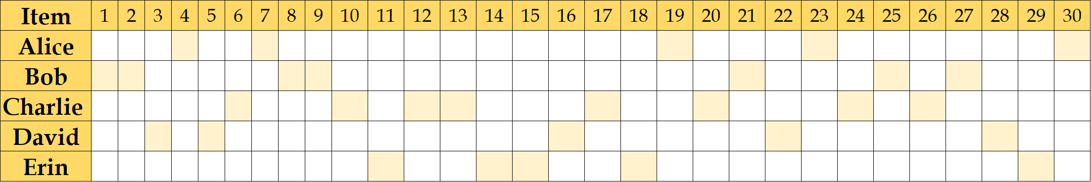
Figure 12: New Allocation Result for 5 researchers

6.2. Fairness Assessment

Recall that in 3.2, expression determining \( σ \) ’s value and \( φ \) ’s value are defined.

6.2.1. Assessment based on pure amount equality

Table 2: \( {σ_{1}} \) and \( {φ_{1}} \) Value

\( {φ_{1}} \lt {σ_{1}} \) , therefore this allocation is fair according to the criteria of pure amount.

6.2.2. Assessment based on the Veil of Ignorance

Table 3: \( {σ_{2}} \) and \( {φ_{2}} \) Value

\( {φ_{2}} \gt 2{σ_{1}} \) , therefore this allocation is unfair according to the criteria of the Veil of Ignorance.

6.2.3. Assessment based on amount equality and the Veil of Ignorance

Table 4: \( {σ_{3}} \) and \( {φ_{3}} \) Value

Table 5: \( α \) Value

\( 0 \lt α \lt 5 \) , therefore this allocation is relatively unfair according to the criteria of amount equality and the Veil of Ignorance

6.2.4. Assessment Based on Utilitarianism

Table 6: \( {σ_{4}} \) and \( {φ_{4}} \) Value

\( {φ_{4}} \lt {σ_{4}} \) , therefore this allocation is fair according to the criteria of Utilitarianism

6.3. Allocation Summary

Under different definitions of fairness, the result varies, but with improved algorithm that includes the Veil of ignorance and the complementation items, the allocations achieve fairness in the majority of definitions. For some cases, the results appear to be unfair because Alice’s estimations are generally low. The table below summarize the fairness with different definitions.

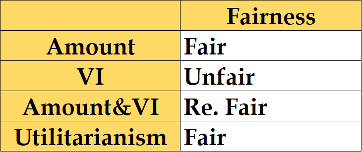
Figure 13: Summary for Allocation Fairness

7. Conclusion

This paper aims to create a thorough and quantitative methodology for allocating resources to reach fairness. By considering several standards of fairness in the beginning, the model successfully quantifies the concepts to mathematics expression. Tangling the tasks, we gradually extend our model into more complicated scenes. The model also simulates the potential social impacts, which discuss how the distribution will be affected, by introducing social behavior, like auction, and preference. Though the results couldn’t be equal for every member, the model manages to reach the fairness, based on our standard, in a maximum degree. The budget constraint is altered, proving the basic versatility of our model.

References

[1]. Mill, J. S. (1863). Utilitarianism. London : Parker, Son and Bourn.
[2]. Rawls, J. (1999). A theory of justice. In Harvard University Press eBooks.
[3]. Piacquadio, P. G. (2017). A fairness justification of utilitarianism. Econometrica, 85(4), 1261–1276.
[4]. Huang, K., Greene, J. D., & Bazerman, M. H. (2019). Veil-of-ignorance reasoning favors the greater good. Proceedings of the National Academy of Sciences of the United States of America, 116(48), 23989–23995.
[5]. Scanlon, T. M. (1977). Rights, goals, and fairness. Erkenntnis, 11(1), 81–95.
[6]. Krawczyk, M. (2009). A model of procedural and distributive fairness. Theory and Decision, 70(1), 111–128.
[7]. Schrijver, A. (2000). Theory of linear and Integer Programming. Journal of the Operational Research Society, 51(7), 892.
[8]. Wasserman, S., & Faust, K. (1994). Social Network Analysis: methods and applications.
Cite this article
Niu,J.;Wang,Z.;Ning,B.;Yang,W.;Sun,X. (2024). Allocation under Justice. Advances in Economics, Management and Political Sciences,88,51-65.
Data availability
The datasets used and/or analyzed during the current study will be available from the authors upon reasonable request.
Disclaimer/Publisher's Note
The statements, opinions and data contained in all publications are solely those of the individual author(s) and contributor(s) and not of EWA Publishing and/or the editor(s). EWA Publishing and/or the editor(s) disclaim responsibility for any injury to people or property resulting from any ideas, methods, instructions or products referred to in the content.
About volume
Volume title: Proceedings of the 2nd International Conference on Management Research and Economic Development
© 2024 by the author(s). Licensee EWA Publishing, Oxford, UK. This article is an open access article distributed under the terms and
conditions of the Creative Commons Attribution (CC BY) license. Authors who
publish this series agree to the following terms:
1. Authors retain copyright and grant the series right of first publication with the work simultaneously licensed under a Creative Commons
Attribution License that allows others to share the work with an acknowledgment of the work's authorship and initial publication in this
series.
2. Authors are able to enter into separate, additional contractual arrangements for the non-exclusive distribution of the series's published
version of the work (e.g., post it to an institutional repository or publish it in a book), with an acknowledgment of its initial
publication in this series.
3. Authors are permitted and encouraged to post their work online (e.g., in institutional repositories or on their website) prior to and
during the submission process, as it can lead to productive exchanges, as well as earlier and greater citation of published work (See
Open access policy for details).