1. Introduction

The COVID-19 pandemic has brought about significant turmoil and uncertainty in global financial markets [1]. During this period, panic among individuals triggered sustained plunges in global stock markets. Unprecedentedly, the US stock market experienced four "circuit breaker" triggers on March 9th, 12th, 16th, and 18th, due to the extreme market volatility [2]. Faced with the economic recession caused by the COVID-19 pandemic, the US government and other countries implemented large-scale fiscal stimulus measures [3]. The successful development and widespread vaccination of vaccines, along with improvements in corporate performance, boosted investor sentiment and greatly restored market confidence. Consequently, the US stock market rebounded significantly after a massive retreat [4].

In this context, portfolio management becomes more complex and crucial. Investors need to reassess the balance between risk and return to cope with market uncertainty and volatility. At the same time, investors need to remain vigilant and adjust their investment strategies promptly according to market changes.

This paper aims to match the optimal portfolio for investors with different risk-aversion levels by modeling and analyzing data from fourteen US technology stocks. Initially, Monte Carlo Simulation is utilized for determine the portfolio’s Efficient Frontier. Then, Minimum Volatility and Maximum Sharpe Ratio portfolios are identified, and their related data are analyzed. Finally, the optimal investment portfolios for investors with different risk aversion levels are derived. The analysis and management of portfolios in this paper is of significant importance in reality, especially during periods of market volatility, which can help investors make better portfolio allocations.

The of the paper’s remaining portion is organized in the following manner. Section 2 presents the data, empirical model, and results analysis. Section 3 shows some limitations. Section 4 concludes the study.

2. Model Formulation

2.1. Application of Markowitz Efficient Frontier

Nobel Laureate Harry Markowitz introduced the concept of the efficient frontier in 1952, which continues to be a core premise of modern portfolio theory. It assesses portfolio based on their balance of return (y-axis) and risk (x-axis). An investor's choices for balancing portfolio risks and returns are graphically illustrated by this efficient frontier [5].

The formulas of expected portfolio return and are as follow:

$E({R_{p}})={w_{1}}​{R_{1}}​+{w_{2}}​{R_{2}}+…+{w_{n}}​{R_{n}}​=\sum _{i=1}^{n}{w_{i}}​{R_{i}}\ \ \ （1）$

$σ_{p}^{2}=\sum _{i=1}^{n}{\sum _{j=1}^{n}{w_{i}}​w_{j}}​{σ_{ij}}\ \ \ (2)$

$E({R_{p}})$ denotes the expected portfolio return, ${R_{i}}$ denotes the expected return of the $i$ th asset, $σ_{p}^{2}$ denotes portfolio’s total risk which measured as variance, ${σ_{ij}}$ denotes the covariance between the $i$ th and $j$ th assets, ${w_{i}}$ denotes the weight of the $i$ th asset in the portfolio, ${w_{j}}$ denotes the weight of the $j$ th asset in the portfolio and $n$ denotes portfolio’s total number of assets.

Modern portfolio theory's Efficient Frontier consists of optimal portfolios which offer the greatest expected return when a certain risk degree is taken into account, or the lowest risk when a defined expected return is taken into account [6]. Portfolios that are located beneath the efficient frontier are judged imperfect since they fail to give enough return regarding the quantity of risk taken. On the contrary, portfolios locate at Efficient Frontier’s right side are also imperfect because more risk is borne for the expected return.

This paper constructs the Efficient Frontier of a portfolio using the daily compounded returns of fourteen US technology stocks, aiming to utilize the efficient frontier for risk management and asset allocation decisions.

2.2. Finding the Efficient Frontier using Monte Carlo Simulation

Monte Carlo Simulation involves mathematical methods that utilized to estimate the potential outcomes of uncertain events and evaluate their risk impacts in various real-world scenarios [7]. It models potential outcomes by utilizing probability distributions for variables with inherent uncertainty and recalculates results using different sets of random numbers within specified ranges. This computation is typically repeated thousands of times to generate a large number of possible outcomes. Due to its high precision, Monte Carlo Simulation is suitable for long-term predictions, and with an increase in the number of inputs, the number of predictions also increases, enabling higher accuracy in predicting results over longer timeframes.

In Monte Carlo simulations, the portfolio’s expected return and variance are estimated using samples of returns generated across numerous simulations:

$E({R_{p}})≈\frac{1}{N}\sum _{i=1}^{n}{R_{p,i}}\ \ \ (3)$

$σ_{p}^{2}≈\frac{1}{N-1}\sum _{i=1}^{n}{({R_{p,i}}​{-E(R_{p}}))^{2}}\ \ \ (4)$

$E({R_{p}})$ denotes the expected portfolio return. ${R_{p,i}}$ denotes the return of portfolio in the $i$ th simulation, $σ_{p}^{2}$ denotes the total risk of the portfolio and $N$ denotes the number of simulations.

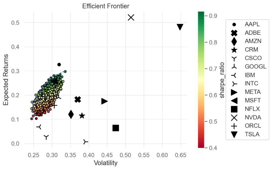
Figure 1: The efficient frontier driven through Monte Carlo Simulation.

Figure 1 displays the efficient frontier of a portfolio consisting of fourteen stocks, which is constructed through Monte Carlo Simulation. NVDA and TSLA exhibit higher expected returns, while IBM and CSCO have lower volatility.

2.3. Discovering Portfolio Performance that has Maximum Sharpe Ratio and Minimum Volatility.

Sharpe ratio refers to the ratio of the portfolio's risk premium to total risk. If the Sharpe ratio is higher, it implies that the portfolio has obtained greater returns though assuming less risk, which means investors have obtained higher returns per unit of risk taken [8]. This makes the Sharpe ratio an important metric for investors who want to maximize their returns in relation to the risks they are taking. By comparing the Sharpe ratios of different investments, investors can identify which portfolios are effectively generating superior risk-adjusted returns.

The following is the formula for Sharpe ratio:

$S=\frac{{R_{p}}-{R_{f}}}{{σ_{p}}}\ \ \ (5)$

$S$ signifies the Sharpe ratio, ${σ_{p}}$ signifies the portfolio volatility, ${R_{p}}$ signifies the portfolio return and ${R_{f}}$ signifies the risk-free rate.

The Efficient Frontier theory defines volatility as standard deviation, which is the difference between returns and their average, often expressed in annualized form [9]. At a certain level of risk, elevating the portfolio’s Sharpe ratio is an objective of the Efficient Frontier theory. To achieve portfolio optimization, investors can identify asset combinations in the portfolio with the highest risk-adjusted returns. This paper constructs graphs for portfolios of Maximizing Sharpe Ratio and Minimum Volatility using Python code, as shown in Figure 2.

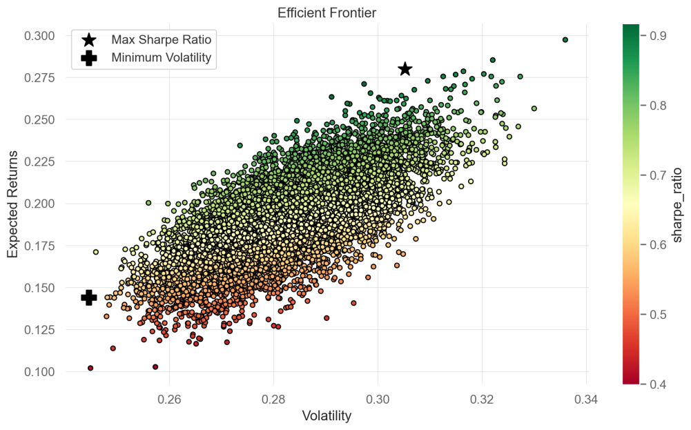
Figure 2: Minimum volatility and Maximum Sharpe Ratio

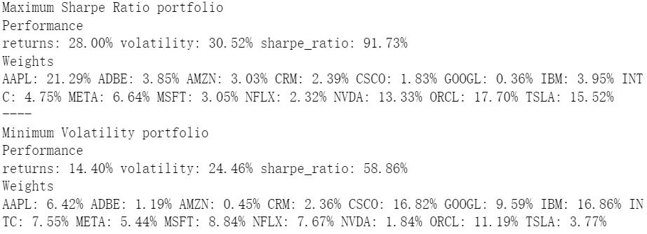
Figure 3: Information about the portfolios.

Figure 3 reveals that the Maximum Sharpe Ratio portfolio's return was 28.00% from January 1, 2019 to December 31, 2023, while that of Minimum Volatility portfolio was 14.40%. Maximum Sharpe Ratio portfolio is typically considered the choice for maximizing returns within an acceptable level of risk. It offers a disciplined approach to balancing high returns with acceptable risk levels, often leading to effective diversification. Therefore, the Maximum Sharpe Ratio of the portfolio consisting of these fourteen technology stocks is 91.73%, with a return of 28.00%. Conversely, to reduce portfolio risk, the Minimum Volatility portfolio is typically chosen by risk-averse investors. It provides more predictable performance, which can be comforting to investors during turbulent market conditions. Thus, the Minimum Volatility of the portfolio consisting of these fourteen technology stocks is 24.46%, with a return of 14.40%.

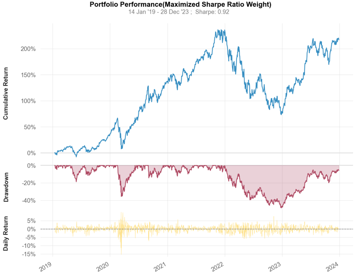
Figure 4: Portfolio performance (Maximum Sharpe Ratio Weight).

Table 1: Some indicators of the Maximum Sharpe Ratio portfolio performance.

Figure 4 represents Maximum Sharpe Ratio portfolio’s cumulative return, drawdown, and daily average return between January 1, 2019 and December 31, 2023. Table 1 shows some parameters of this portfolio.

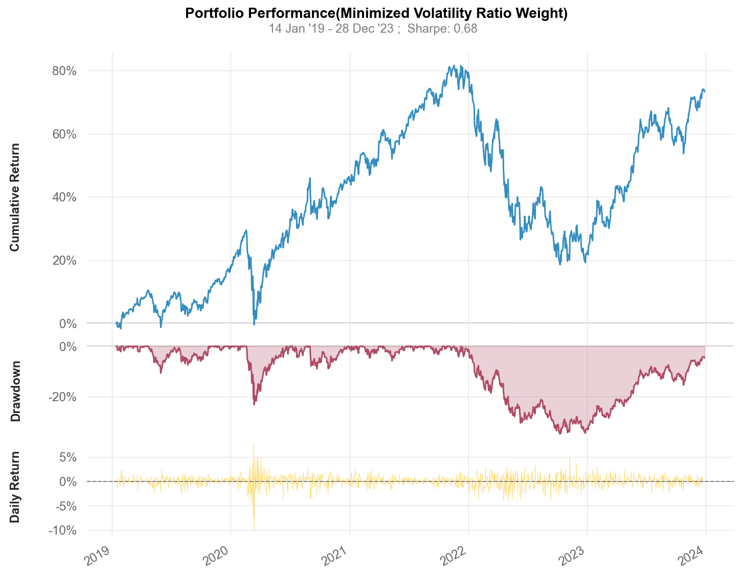
Figure 5: Portfolio performance (Minimum Volatility Weight).

Table 2: Some indicators of the Minimum volatility portfolio performance.

Figure 5 represents Minimum Volatility portfolio’s cumulative return, drawdown, and daily average return between January 1, 2019 and December 31, 2023. Table 2 shows some parameters of this portfolio.

Maximum Sharpe Ratio portfolio performed better than Minimum Volatility portfolio regarding annual and cumulative return, as determined by the comparison. However, Maximum Sharpe Ratio portfolio had a larger maximum drawdown than the Minimum Volatility portfolio due to its higher annual volatility. This indicates that the higher risks are associated with higher potential returns. By pursuing the optimal risk-return trade-off, the Maximum Sharpe Ratio portfolio is willing to compromise greater volatility and potential drawdowns for higher returns. Conversely, the Minimum Volatility portfolio offers greater security and stability, though this comes at the expense of diminished growth potential.

2.4. Analyzing Portfolio Allocation based on Risk Aversion Levels

Risk aversion is crucial as it determines how sensitive an investor is to changes in risk. Investors prioritize either stability or higher returns based on their financial objectives and individual comfort with uncertainty. Different investors have varying perceptions and tolerance levels towards risk, leading to different degrees of risk aversion. [10] Investors who are risk-averse typically prefer returns that are more certain, even if they may have a lower expected return, which primarily due to their inherent need for security and fear of potential losses. Conversely, the non-risk-averse investors are less impacted by potential negative outcomes and are more focused on the potential for significant gains.

Figure 6 shows the allocation of asset weights at different levels of risk aversion (represented by γ), indicating the portfolio compositions that aim to achieve maximum returns at specific levels of risk aversion.

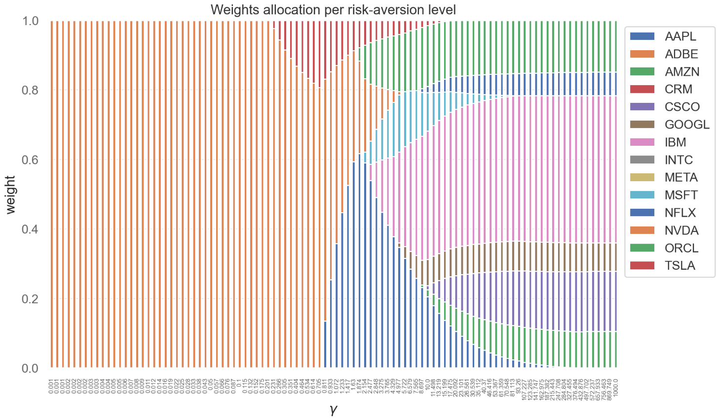
Figure 6: Weight allocation per risk-aversion level.

Through analysis of Figure 6, we can draw the following conclusions. When investors have a low level of risk aversion (γ values between 0.001 and 0.705), the portfolio has a higher allocation to NVDA because of its higher volatility and expected return, making it the optimal choice for lower levels of risk aversion. When investors have a high level of risk aversion (γ values between 107.227 and 1000), the portfolio has a significant allocation to IBM and CSCO because of their lower volatility and expected returns, indicating that these assets can effectively control the total portfolio risk. Considering COVID-19 pandemic, investors' risk preferences shifted notably in the short term, and their risk-averse behaviors had significantly increased [11]. Therefore, holding more positions of IBM and CSCO is a defensive, investment strategy which reduces exposure to high-volatility assets and increases diversification during periods of high risk-aversion.

3. Limitations

Due to various assumptions underlying the Efficient Frontier Theory, such as the consideration of risk-return trade-offs by investors in the process of deciding investment choices, The assumption of market efficiency and the positive correlation between risk and return may not be completely accurate in real markets, resulting in deviations from the results of this paper and actual circumstances. Additionally, the data period of this paper spans from January 1, 2019, to December 31, 2023, whereas the Efficient Frontier Theory typically requires data covering multiple market cycles to ensure representativeness. Therefore, four years of asset return data may not be sufficiently comprehensive. Furthermore, transaction costs, agency costs, and other frictions occur in actual markets are not factored into this paper, resulting in ideal rather than realistic outcomes.

4. Conclusions

This paper collected the return data of fourteen US technology stocks from January 1, 2019, to December 31, 2023, and successfully derived the Efficient Frontier of the investment portfolio using Monte Carlo Simulation. Minimum Volatility and Maximum Sharpe Ratio portfolio allocations were determined by this paper, and it discovered that greater volatility and potential drawdowns come at the cost of the possibility of higher returns. In contract, the diminished growth potential is the expense of greater security and stability. Furthermore, the paper concluded the optimal portfolio allocation considering investors with different risk aversion, revealing that when investors have a lower risk aversion, the portfolio has a higher allocation of NVDA due to its higher volatility and expected return. Conversely, when investors have a higher risk aversion, IBM and CSCO have a larger allocation as their lower volatility effectively controls the overall portfolio risk. In the context of COVID-19 pandemic when investors’ risk-averse behaviors had significantly increased. Holding more positions of IBM and CSCO is a defensive strategy which reduces exposure to high-volatility assets and increase diversification. However, due to the Efficient Frontier Theory being based on various assumptions and the existence of transaction costs in reality, the analysis in this paper still has limitations and uncertainties. In the future, analysts should use more precise models to analyze the data and attempt to quantify the uncertainty factors as much as possible.

References

[1]. Li Y, Zhuang X, Wang J, et al. Analysis of the impact of COVID-19 pandemic on G20 stock markets[J]. The North American Journal of Economics and Finance, 2021, 58: 101530.
[2]. Bai L, Wei Y, Wei G, et al. Infectious disease pandemic and permanent volatility of international stock markets: A long-term perspective[J]. Finance research letters, 2021, 40: 101709.
[3]. Wilson D J. The covid-19 fiscal multiplier: Lessons from the great recession[J]. FRBSF Economic Letter, 2020, 13: 1-5.
[4]. Guan C, Liu W, Cheng J Y C. Using social media to predict the stock market crash and rebound amid the pandemic: the digital ‘haves’ and ‘have-mores’[J]. Annals of Data Science, 2022, 9(1): 5-31.
[5]. Alexander N, Scherer W, Burkett M. Extending the Markowitz model with dimensionality reduction: Forecasting efficient frontiers[C]//2021 Systems and Information Engineering Design Symposium (SIEDS). IEEE, 2021: 1-6.
[6]. Parkinson, Charity Smith, "Maximizing Returns for Investors Using Modern Portfolio Theory and the Efffcient Frontier" (2020). Undergraduate Honors Capstone Projects. 494.
[7]. Raychaudhuri S. Introduction to monte carlo simulation[C]//2008 Winter simulation conference. IEEE, 2008: 91-100.
[8]. Kourtis A. The Sharpe ratio of estimated efficient portfolios[J]. Finance Research Letters, 2016, 17: 72-78.
[9]. Zhang L, Li D, Lai Y. Equilibrium investment strategy for a defined contribution pension plan under stochastic interest rate and stochastic volatility[J]. Journal of Computational and Applied Mathematics, 2020, 368: 112536.
[10]. O'Donoghue T, Somerville J. Modeling risk aversion in economics[J]. Journal of Economic Perspectives, 2018, 32(2): 91-114.
[11]. Nisani D, Qadan M, Shelef A. Risk and Uncertainty at the Outbreak of the COVID-19 Pandemic[J]. Sustainability, 2022, 14(14): 8527.
Cite this article
Lyu,Y. (2024). Empirical Analysis of Portfolio Allocation During Market Turbulence Based on Efficient Frontier. Advances in Economics, Management and Political Sciences,110,85-92.
Data availability
The datasets used and/or analyzed during the current study will be available from the authors upon reasonable request.
Disclaimer/Publisher's Note
The statements, opinions and data contained in all publications are solely those of the individual author(s) and contributor(s) and not of EWA Publishing and/or the editor(s). EWA Publishing and/or the editor(s) disclaim responsibility for any injury to people or property resulting from any ideas, methods, instructions or products referred to in the content.
About volume
Volume title: Proceedings of ICEMGD 2024 Workshop: Decoupling Corporate Finance Implications of Firm Climate Action
© 2024 by the author(s). Licensee EWA Publishing, Oxford, UK. This article is an open access article distributed under the terms and
conditions of the Creative Commons Attribution (CC BY) license. Authors who
publish this series agree to the following terms:
1. Authors retain copyright and grant the series right of first publication with the work simultaneously licensed under a Creative Commons
Attribution License that allows others to share the work with an acknowledgment of the work's authorship and initial publication in this
series.
2. Authors are able to enter into separate, additional contractual arrangements for the non-exclusive distribution of the series's published
version of the work (e.g., post it to an institutional repository or publish it in a book), with an acknowledgment of its initial
publication in this series.
3. Authors are permitted and encouraged to post their work online (e.g., in institutional repositories or on their website) prior to and
during the submission process, as it can lead to productive exchanges, as well as earlier and greater citation of published work (See
Open access policy for details).