


1. Introduction
An investment portfolio is a specific allocation of financial assets designed to stabilize the risk of underperformance across different investment pools [1]. Selecting assets for the portfolio is crucial for investors and financial institutions. It is also difficult because it involves making decisions under conditions of uncertainty [2]. The varying levels of expected risk associated with different securities prompt most investors to consider holding a diverse portfolio. This strategy aims to mitigate risk by avoiding the concentration of investments in a single security, effectively spreading the risk across multiple assets [1]. As a result, what investors and firms care most about is making their combination of assets generate higher returns with lower risk.
In 1952, Markowitz introduced Modern Portfolio Theory and popularized efficient portfolio selection methods [3]. The theory revolutionized finance by introducing a quantitative framework for maximizing returns while minimizing risk through diversification. Markowitz's portfolio theory was the foundation for the development of the Capital Asset Pricing Model (CAPM) a decade later. It was a significant innovation in finance and business at a time when the theoretical frameworks for choice-making under uncertainty had already been developed and widely embraced, as it incorporated risk and return in a linear relationship [4]. The predictive potential of the Fama-French Factor Model is enhanced by the inclusion of additional factors, which is an extension of the Capital Asset Pricing Model (CAPM). Karp and Vuuren examined the validity and effectiveness of CAPM and the Fama French Three-Factor Model in predicting returns and variations [5]. More recently, Chen, Pelger, and Zhu studied the application of deep learning in asset pricing and proposed a new asset pricing model, while Heaton, Polson, and Witte discussed methods for constructing financial portfolios using deep learning [6-7]. Rasekhschaffe and Jones explored the application of machine learning to portfolio selection and evaluated its predictive performance [8]. LightGBM was talked about by Ke, Meng, Finley, Wang, Chen, Ma, Ye, and Liu [9]. They used it to quickly train on large datasets and showed two new techniques that make gradient-boosting decision trees (GBDT) work better: gradient-based one-side sampling (GOSS) and exclusive feature bundling (EFB). Over the past few years, LightGBM has been extensively employed in various machine learning applications and multiple research fields due to its advantages in large-scale data processing and efficient model building, such as finance, quality inspection, crop breeding, and so on. It has become a hot research topic, although the research introducing LightGBM into return prediction and portfolio allocation is still relatively limited.
This research aims to connect the more traditional Fama-French three-factor model and the newer LightGBM method with return prediction and portfolio management to facilitate more effective asset allocation strategies. To accomplish this goal, this article first selects eight top-performing assets from different industry sectors. The adjusted closing prices are converted to daily returns. This study then uses the previous five years of stock price data to train a Fama-French three-factor model and a LightGBM model to directly project the next whole year’s stock returns at once. The mean-variance model and Monte Carlo simulation are used to create an efficient frontier and obtain the maximum Sharpe ratio allocation and minimum risk allocation. Lastly, by applying real-life data to the generated weights, the cumulative returns of four models are calculated and compared with the benchmark S&P 500’s cumulative returns.
The remainder of this paper is structured as follows: Section 2 shows the data utilized in this research and explains the asset selection process, providing a descriptive overview of the chosen stocks. Section 3 delves into the methodologies applied, including the Fama-French Factor Model, LightGBM, Monte Carlo Simulation, and other techniques. Section 4 evaluates the effectiveness of the proposed approach, creating efficient frontiers and generating four optimal portfolios, and compares the results with the benchmark S&P 500. Lastly, the paper is concluded in Section 5, which proposes potential areas for future research.
2. Data Source and Pre-process
Eight representative assets have been selected for the portfolio: NVDA, MSFT, NFLX, FSLR, COST, GE, PGR, and IWM (See Table 1). These assets are chosen due to their status as top performers in categories such as blue-chip technology stocks, high momentum stocks, non-cyclical stocks, and small-cap stock ETFs. The portfolio, characterized by high growth potential and strong diversification, aims to exceed the cumulative return of the S&P 500 index.
Table 1: Selected assets
Asset Symbol | Company |
NVDA | NVIDIA Corporation |
MSFT | Microsoft Corporation |
NFLX | Netflix, Inc. |
FSLR | First Solar, Inc. |
COST | Costco Wholesale Corporation |
GE | General Electric Company |
PGR | The Progressive Corporation |
IWM | The iShares Russell 2000 ETF |
The asset data utilized in this analysis is sourced from Yahoo Finance (https://finance.yahoo.com/). Adjusted close price data collected from April 30, 2018, to April 30, 2023, serves as the training set, while adjusted close price data from May 1, 2023, to May 1, 2024, constitutes the test set. In total, 1259 rows of data are collected, and 252 market days are examined. Adjusted close prices are transferred into daily returns based on formula (1), and basic information is shown in Table 2.
rt=Pt−Pt−1Pt−1 | (1) |
Table 2: Descriptive statistics of five stocks
index | mean | std | skew | kurtosis |
COST | 0.00092 | 0.01533 | -0.18601 | 8.76923 |
FSLR | 0.00121 | 0.03035 | 0.16206 | 2.99979 |
GE | 0.00053 | 0.02727 | 0.11421 | 4.07668 |
IWM | 0.00030 | 0.01672 | -0.68839 | 7.47580 |
MSFT | 0.00118 | 0.01957 | 0.00802 | 6.66944 |
NFLX | 0.00050 | 0.02972 | -1.31042 | 19.29019 |
NVDA | 0.00182 | 0.03292 | -0.16057 | 3.18489 |
PGR | 0.00091 | 0.01684 | 0.02942 | 5.84100 |
3. Method
Four main steps are performed, as shown in Figure 1. Firstly, this study selects eight top performers from different sectors. Secondly, the study trains a Fama French Three Factor model and a LightGBM model using data from April 30, 2018, to April 30, 2023, to predict stock returns from May 1, 2023, to May 1, 2024, at once. Thirdly, mean-variance analysis and the Mento Carlo model are applied to create efficient frontiers and calculate optimal portfolio weights. Totally, four options are presented. Lastly, the study evaluates based on real data and compares the performance of four portfolios and the benchmark S&P 500 index.
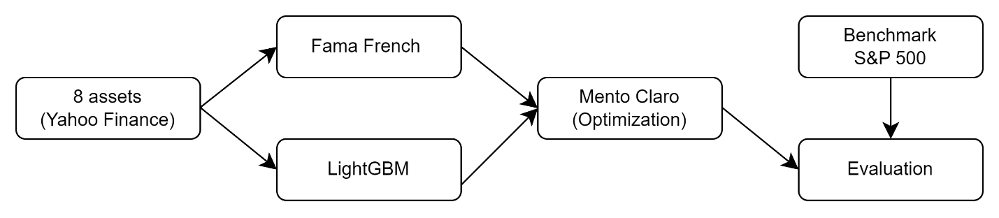
Figure 1: Basic Steps of the Study
3.1. Mean Variance Model
The mean variance model is a modern portfolio theory framework developed by Harry Markowitz in 1952. It is a crucial and fundamental model because it helps optimize portfolios by maximizing returns for a given level of risk, effectively balancing the tradeoff between risk and return, and explaining the benefits of diversification. The weighted mean of the projected returns of all the assets in a portfolio is the portfolio's expected return.
E({r_{p}})=\sum _{i=1}^{N}{w_{i}}*{μ_{i}} | (2) |
{μ_{i}} denotes as expected return of each asset which are already defined in data section above. {w_{i}} denotes as weight for the i-th asset. Variance measures the risk of a portfolio. It shows the dispersion of returns compared to expected returns.
σ_{p}^{2}=\sum _{i=1}^{N}\sum _{j=1}^{N}{w_{i}}*{w_{i}}*{σ_{ij}} | (3) |
{σ_{p}}=\sqrt[]{σ_{p}^{2}} | (4) |
σ_{p}^{2} and {σ_{p}} represents the variance and risk of a portfolio, and {σ_{ij}} represents the covariance between two asset returns and how two returns move together.
Sharpe ratio is one of the best measures of risk-adjusted return and helps investors understand the portfolio’s return in relation to its risk. It is a key metric for measuring the performance of different portfolios and constructing optimal portfolios, even when the risks are different.
Sharpe Ratio= \frac{{r_{p}}-{r_{f}}}{{σ_{p}}} | (5) |
{r_{f}} is the market risk-free rate. This study compares performance of maximum Sharpe ratio portfolio with minimum volatility portfolio and benchmark S&P500.
3.2. Mento Carto Simulation
The capacity of Mento Carlo Simulation to handle uncertainty, allow incorporation of complex model, and facilitate scenario analysis led to its widespread use in finding the efficient frontier and portfolio optimization [10] (See Figure 2).
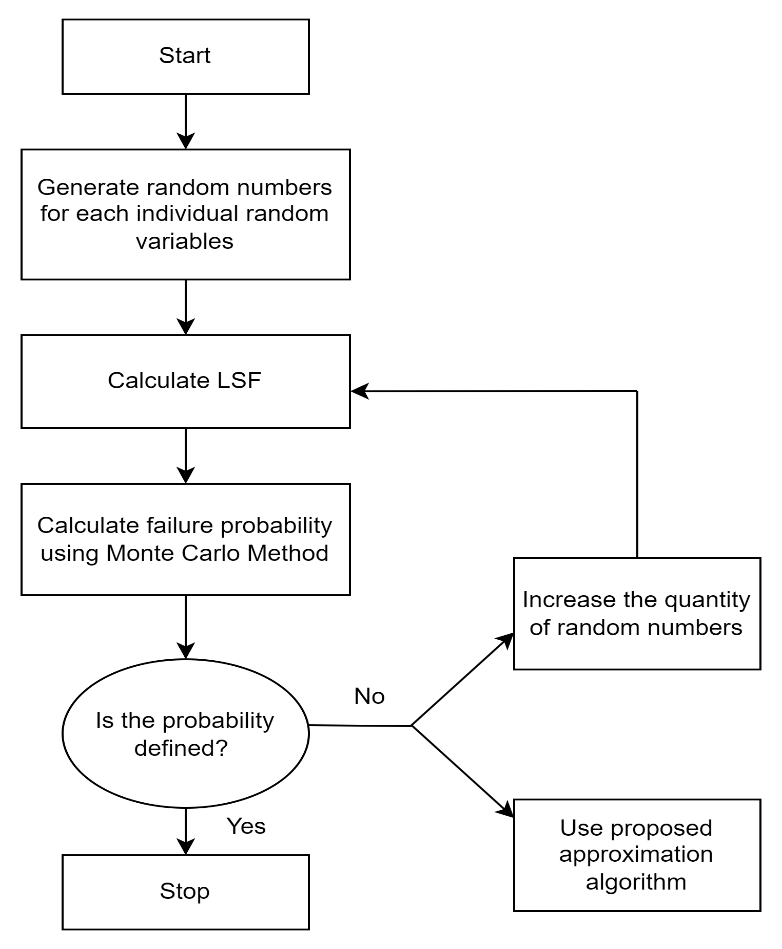
Figure 2: Mento Carlo Algorithm
Random weights ( {w_{i}}) are generated and assigned for each asset to create random portfolios with sum of weights equals to one.
\sum _{i=1}^{N}{w_{i}}=1 | (6) |
By generating a large quantity of random portfolios and plotting random portfolios on a risk return graph, efficient frontier can be generated and two optimal portfolios (the minimum volatility portfolio and the maximum Shape ratio portfolio) can be identified. Then, the expected return, volatility, and Sharpe Ratio are calculated as described in Mean-Variance Model.
3.3. Fama-French Three Factor Model
Ken French and Eugene Fama, two renowned researchers who conducted significant work in the field of factor modeling, identified "value" and "size" as two crucial factors in explaining asset returns, in addition to market risk (MKT) [11]. They specifically introduced the SMB (Small Minus Big) factor to account for size risk and the HML (High Minus Low) factor to address value risk [11]. The Fama-French three-factor model is expressed as:
{r_{A}}={r_{f}}+{β_{A}}MKT+{s_{A}}SMB+{h_{A}}HML | (7) |
The MKT factor represents the additional returns expected from investing in a risky market portfolio compared to risk-free assets.
SMB measures the difference (typically positive) in returns between stocks with a modest market capitalization and those with a large market capitalization. Typically, small-cap stocks are considered to be riskier with higher growth potential. SMB captures the expected premium for the additional risk investors take with small companies.
HML indicates the difference in returns between stocks of companies with a high book-to-market ratio (value stocks) and those with a low book-to-market ratio (growth stocks).
In this formula (7), {β_{A}} , {s_{A}} , and {h_{A}} are the coefficients for the three factors, reflecting the asset's sensitivity to each factor.
Fama-French is one of the most commonly used models because of its ability to predict asset returns more accurately than traditional CAPM. It’s three factors consistently demonstrated the highest predictive power (often resulting in an R-square value around 95%) among any other factors tested by researchers [11].
3.4. LightGBM (Light Gradient Boosting Machine)
LightGBM is an efficient and accurate machine learning algorithm developed by Microsoft. It is mainly based on gradient boosting framework and uses a histogram-based algorithm, efficiently handling large quantities of data and reducing complexity.
Initialization: Start with initial prediction {\hat{{y_{i}}}^{(0)}} which is the mean of returns across all training samples
Gradient calculation: Compute negative residuals for current predictions:
g_{i}^{(t)}= -\frac{∂L({y_{i}},{\hat{{y_{i}}}^{(t-1)}})}{∂{\hat{{y_{i}}}^{(t-1)}}} | (8) |
L is the loss function, {y_{i}} is the actual return for i-th sample, and {\hat{{y_{i}}}^{(t-1)}} is the predicted returns from previous iteration (t-1).
Histogram-based decision tree learning: Convert continuous features into discrete bins, and for each feature value, calculate hessian and gradient statistics and create histograms.
Find the Best Splits: Calculate information gain for each possible split:
Information Gain={Gain_{left}}+{Gain_{right}}-{Gain_{parent}} | (9) |
Choosing the maximized information gain split refers as Leaf-wise Growth, providing more efficiency and accuracy than traditional level-wise growth.
Update the model: Current prediction is updated by adding a new tree’s prediction scaled by a learning rate:
{\hat{{y_{i}}}^{(t)}}={\hat{{y_{i}}}^{(t-1)}}+ŋ*{f_{t}}({x_{i}}) | (10) |
{\hat{{y_{i}}}^{(t)}} is updated prediction for i-th sample, ŋ is the learning rate, and {f_{t}}({x_{i}}) is newly added tree prediction.
This study contains 1005 data points in the training dataset and 8 features. The total number of bins used for splitting features is 2040. Eight iterations have been successfully completed.
4. Results
Firstly, from the training set (April 30th, 2018, to April 30th, 2023), this study directly projects the next whole year’s (from May 1st, 2023, to May 1st, 2024) stock daily returns at once using Fama-French Three Factor Model and Machine Learning LightGBM, as show in Figures 3 and 4:
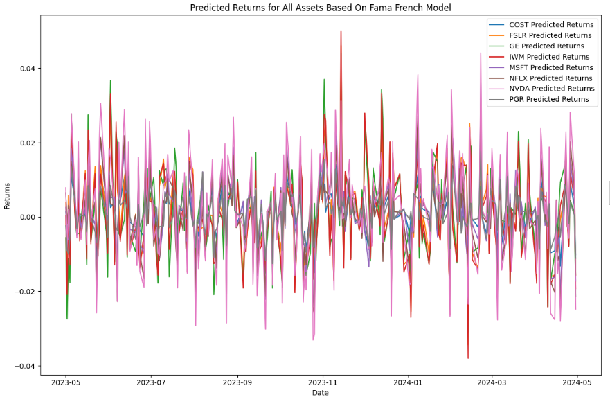
Figure 3: Predicted Returns Based on Fama-French Model
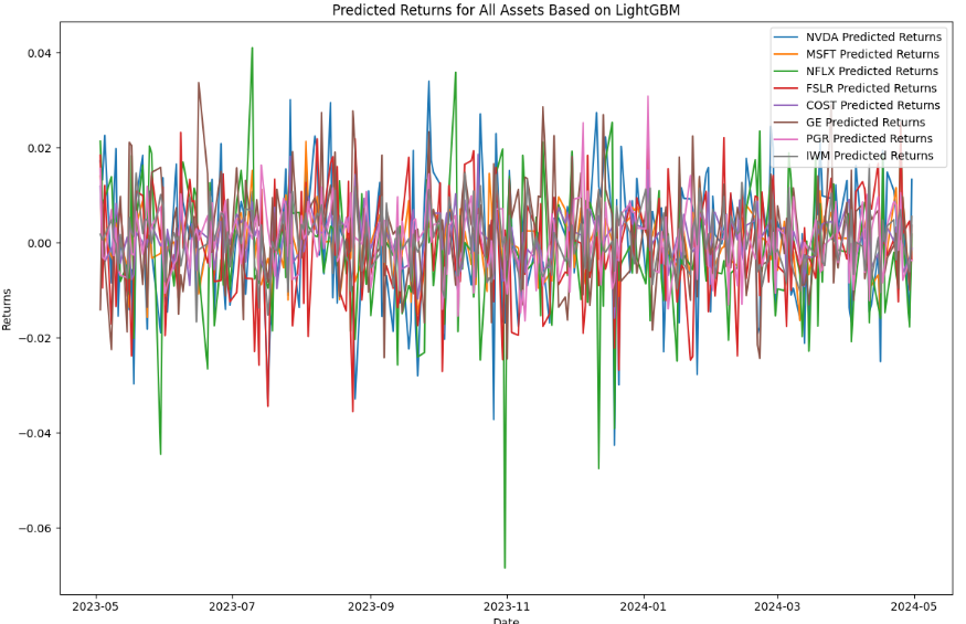
Figure 4: Predicted Returns Based on LightGBM
Based on predicted returns in step one, the Monte Carlo model has been applied to generate 10,000 random portfolios, each with unique weights for both Fama-French and LightGBM predicted returns. Figures 5 and 6 show the expected returns and expected volatility for these portfolios:
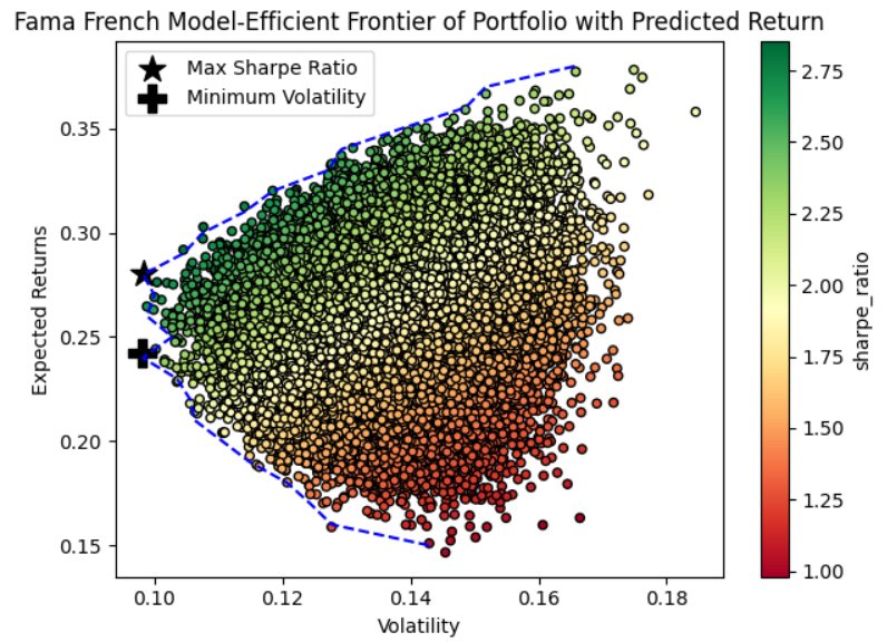
Figure 5: Fama French model-efficient frontier
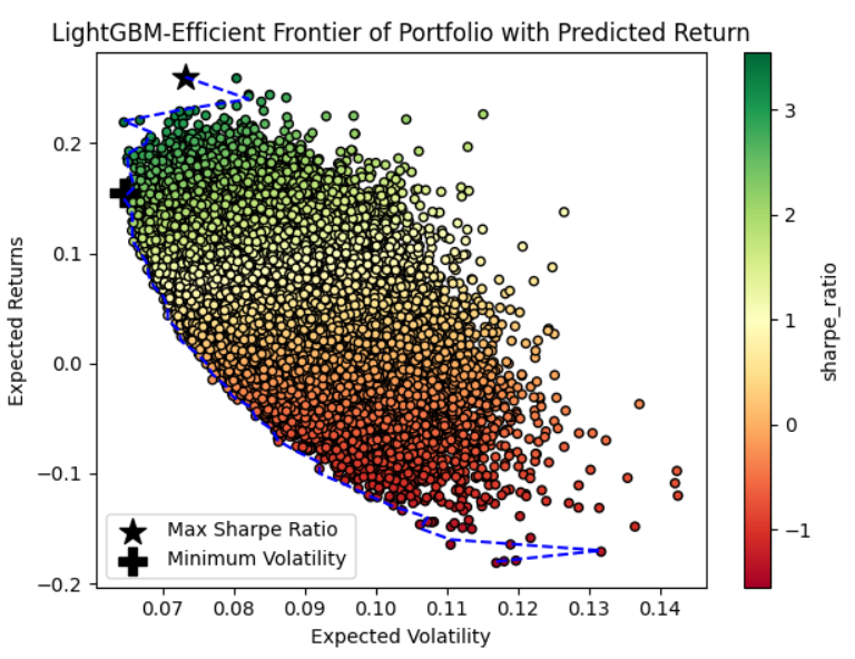
Figure 6: LightGBM-Efficient Frontier
Each circle represents the one random weighted portfolio generated by the Monte Carlo model. Starting from the plus mark, the blue dot line above marks the efficient frontier, the black star mark represents the maximum Sharpe Ratio portfolio combination, and the black plus mark represents the minimum volatility portfolio combination. Four asset allocation options are provided by Mento Carlo Simulation, and specific portfolio weights for each asset are shown in Table 3. The LightGBM-Max Sharpe Ratio portfolio heavily favors Costco (44.28%) and General Electric (25.38%), while the LightGBM-Min Volatility strategy distributes weights more evenly, with significant allocations to Costco (26.76%), Microsoft (21.14%), IWM (18.39%), and Progressive (17.81%). The Fama French-Max Sharpe Ratio portfolio puts heavy weights on NVIDIA (36.59%) and IWM (38.43%), and the Fama French-Min Volatility portfolio also favors NVIDIA (33.25%) and IWM (33.03%) but also includes notable weights for Netflix (16.6%) and General Electric (8.47%).
Table 3: Allocation weights of four portfolios
Allocation options | Weights for each asset | |||||||
NVDA | MSFT | NFLX | FSLR | COST | GE | PGR | IWM | |
LightGBM-Max Shape Ratio | 0.0548 | 0.0412 | 0.0075 | 0.0045 | 0.4428 | 0.2538 | 0.0108 | 0.1847 |
LightGBM-Min Volatility | 0.0045 | 0.2114 | 0.0393 | 0.0108 | 0.2676 | 0.1038 | 0.1781 | 0.1839 |
Fama French-Max Sharpe Ratio | 0.3659 | 0.0288 | 0.1054 | 0.0092 | 0.028 | 0.0142 | 0.064 | 0.3843 |
Fama French-Min Volatility | 0.3325 | 0.0383 | 0.166 | 0.0434 | 0.0031 | 0.0847 | 0.0017 | 0.3303 |
Based on the asset weights, this study evaluates the performance of each portfolio using real-life data from May 1st, 2023, to May 1st, 2024. The results are shown in the following Figure 7 and Table 4:
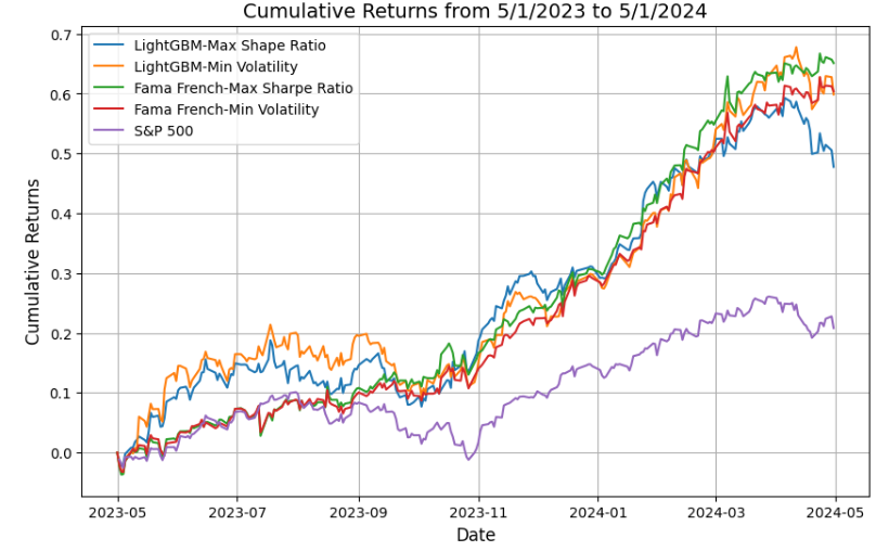
Figure 7: Cumulative Returns of Four Portfolios and S&P 500 Index
Table 4: Statistics of Four Portfolios
Allocation options | Cumulative Returns (%) | Risk (%) | Sharpe Ratio |
LightGBM-Max Shape Ratio | 47.7543 | 17.26 | 2.35 |
LightGBM-Min Volatility | 59.8709 | 19.67 | 2.4852 |
Fama French-Max Sharpe Ratio | 65.1118 | 14.96 | 3.4308 |
Fama French-Min Volatility | 60.4078 | 14.26 | 3.3876 |
S&P 500 | 20.8216 | 11.69 | 1.6832 |
The purple line shows the cumulative returns of the S&P 500; the remaining lines in other colors show the cumulative returns of four portfolio options. All four portfolios clearly and significantly perform better than the benchmark S&P 500.
Based on Table 4, the following traits can be observed:
Although S&P 500 has the lowest volatility (11.69%), its return (20.82%) is significantly lower than other portfolios, causing its Sharpe Ratio (1.68) to also be lower than other options; The LightGBM-Max Sharpe Ratio portfolio is not the optimal option because it has the lowest returns (47.75%) among the four allocation options. It also did poorly on mitigating the volatility (17.26%); LightGBM-Min Volatility Portfolio and Fama French-Min Volatility Portfolio both have returns around 60%, but Fama French-Min Volatility Portfolio (14.26%) mitigates volatility much better than LightGBM-Min Volatility Portfolio (19.67%); The Fama French-Max Sharpe Ratio portfolio has a final overall cumulative return of 65.12% (over 3 times over the S&P 500 index) and a Sharpe Ratio of 3.43 (over 2 times over the S&P 500 index), which are the best among all other portfolios and benchmarks in this study. In Figure 7, the Fama French-Max Sharpe Ratio portfolio also demonstrates the most steady and gradual increase in cumulative returns, whereas other options show more and deeper fluctuation.
5. Conclusion
This research paper presents a novel approach to financial portfolio optimization by integrating the Fama-French model or the LightGBM model. The study uses these models to forecast future stock returns and identify optimal asset allocations that balance maximizing returns with minimizing risks.
Eight high-performing assets are first selected from diverse industry sectors. The Fama-French model and LightGBM model are applied to process and analyze the first 83.33% of the data, followed by making predictions for the subsequent 16.67% in one go. This study then employes mean variance analysis and Monte Carlo simulation to generate the efficient frontier, identifying the maximum Sharpe ratio portfolio and the minimum risk portfolio. The cumulative return sheet clearly demonstrates that the developed portfolios consistently outperform the S&P 500 benchmark. This outcome highlights the effectiveness of combining traditional financial models with advanced machine learning techniques to enhance investment strategies.
In conclusion, the research underscores the practical applications of CPAM and machine learning in financial portfolio management. It affirms the value of this innovative approach for investors and financial institutions seeking to improve their asset allocation processes. However, limitations are presented. Eight assets are chosen, which may not represent the entire market. Other risk factors not considered in the Fama-French model might influence portfolio performance. As the time horizon becomes wider and trading becomes increasingly complex, interpretability and validity can become challenging. In this context, the models utilized in this study hold potential for further refinement and expansion in future research to yield even superior outcomes.
References
[1]. Kapoor, N. (2014). Financial Portfolio management: Overview and Decision Making in investment Process. International Journal of Research (IJR), 1.
[2]. Constantinides, G. M., Malliaris, A. G. (1995). Portfolio Theory. Handbooks in OR & MS, 9.
[3]. Halim, N. A., Yuliati, A. (2020). Markowitz Model Investment Portfolio Optimization: a Review Theory. International Journal of Research in Community Service, 1(3), 14-18.
[4]. Putra, J. M., Soehaditama, J. P., Hernawan, M. A., Yulihapsari, I. U., Sova, M. (2023). Implementing the Capital Asset Pricing Model in Forecasting Stock Returns: A Literature Review. Indonesian Journal of Business Analytics (IJBA), 3(2), 171-182.
[5]. Karp, A., & Vuuren, G. V. (2017). The capital asset pricing model and fama-french three factor model in an emerging market environment. International Business & Economics Research Journal, 16(3).
[6]. Chen, L., Pelger, M., & Zhu, J. (2021). Deep Learning in Asset Pricing. Journal of Financial Economics, 142(3), 994-1015.
[7]. Heaton, J. B., Polson, N. G., & Witte, J. H. (2017). Deep learning for finance: deep portfolios. Applied Stochastic Models in Business and Industry, 33(1), 3-12.
[8]. Rasekhschaffe, K. C., & Jones, R. (2019). Machine learning for stock selection. Financial Analysts Journal, 75(3), 70-88.
[9]. Ke, G., Meng, Q., Finley, T., Wang, T., Chen, W., Ma, W., Ye, Q., & Liu, T. Y. (2017). LightGBM: A Highly Efficient Gradient Boosting Decision Tree. NIPS, 3149-3157.
[10]. Far, M. S., & Wang, Y. (2016). Approximation of the Monte Carlo Sampling Method for Reluability Analysis of Structures. Reasearhgate, 9.
[11]. Kent, L. W., & Ying, Z. (2003). Understanding Risk and Return, the CAPM, and the Fama-French Three-Factor Model. SSRN.
Cite this article
Xiao,M. (2024). Portfolio Optimization Strategy Based on Fama-French and LightGBM. Advances in Economics, Management and Political Sciences,90,169-179.
Data availability
The datasets used and/or analyzed during the current study will be available from the authors upon reasonable request.
Disclaimer/Publisher's Note
The statements, opinions and data contained in all publications are solely those of the individual author(s) and contributor(s) and not of EWA Publishing and/or the editor(s). EWA Publishing and/or the editor(s) disclaim responsibility for any injury to people or property resulting from any ideas, methods, instructions or products referred to in the content.
About volume
Volume title: Proceedings of the 3rd International Conference on Financial Technology and Business Analysis
© 2024 by the author(s). Licensee EWA Publishing, Oxford, UK. This article is an open access article distributed under the terms and
conditions of the Creative Commons Attribution (CC BY) license. Authors who
publish this series agree to the following terms:
1. Authors retain copyright and grant the series right of first publication with the work simultaneously licensed under a Creative Commons
Attribution License that allows others to share the work with an acknowledgment of the work's authorship and initial publication in this
series.
2. Authors are able to enter into separate, additional contractual arrangements for the non-exclusive distribution of the series's published
version of the work (e.g., post it to an institutional repository or publish it in a book), with an acknowledgment of its initial
publication in this series.
3. Authors are permitted and encouraged to post their work online (e.g., in institutional repositories or on their website) prior to and
during the submission process, as it can lead to productive exchanges, as well as earlier and greater citation of published work (See
Open access policy for details).
References
[1]. Kapoor, N. (2014). Financial Portfolio management: Overview and Decision Making in investment Process. International Journal of Research (IJR), 1.
[2]. Constantinides, G. M., Malliaris, A. G. (1995). Portfolio Theory. Handbooks in OR & MS, 9.
[3]. Halim, N. A., Yuliati, A. (2020). Markowitz Model Investment Portfolio Optimization: a Review Theory. International Journal of Research in Community Service, 1(3), 14-18.
[4]. Putra, J. M., Soehaditama, J. P., Hernawan, M. A., Yulihapsari, I. U., Sova, M. (2023). Implementing the Capital Asset Pricing Model in Forecasting Stock Returns: A Literature Review. Indonesian Journal of Business Analytics (IJBA), 3(2), 171-182.
[5]. Karp, A., & Vuuren, G. V. (2017). The capital asset pricing model and fama-french three factor model in an emerging market environment. International Business & Economics Research Journal, 16(3).
[6]. Chen, L., Pelger, M., & Zhu, J. (2021). Deep Learning in Asset Pricing. Journal of Financial Economics, 142(3), 994-1015.
[7]. Heaton, J. B., Polson, N. G., & Witte, J. H. (2017). Deep learning for finance: deep portfolios. Applied Stochastic Models in Business and Industry, 33(1), 3-12.
[8]. Rasekhschaffe, K. C., & Jones, R. (2019). Machine learning for stock selection. Financial Analysts Journal, 75(3), 70-88.
[9]. Ke, G., Meng, Q., Finley, T., Wang, T., Chen, W., Ma, W., Ye, Q., & Liu, T. Y. (2017). LightGBM: A Highly Efficient Gradient Boosting Decision Tree. NIPS, 3149-3157.
[10]. Far, M. S., & Wang, Y. (2016). Approximation of the Monte Carlo Sampling Method for Reluability Analysis of Structures. Reasearhgate, 9.
[11]. Kent, L. W., & Ying, Z. (2003). Understanding Risk and Return, the CAPM, and the Fama-French Three-Factor Model. SSRN.