1. Introduction

Housing prices have always been a topic worth discussing. For the government, housing prices are a key issue that needs to be monitored. Governments and planners can make more effective decisions on land use policies. Government regulation can significantly improve housing affordability and availability [1]. emphasized the importance of stabilizing the housing market and suggested that targeted government policies can help regulate housing prices and improve the affordability of low-income families. Housing prices are also closely related to a family. The causal chain between housing price changes and observable changes in outcome variables such as economic behavior and consumption requires that individuals at least be able to perceive the impact of housing price changes on their family wealth and recognize the impact on their financial situation [2]. In addition, buying a house is not only a means of obtaining housing but also a major investment. Especially for risk-averse investors, housing can be a beneficial component of a family portfolio [3]. By analyzing market trends and predicting housing prices, people can determine whether a property in a certain location is suitable for investment.

This paper uses machine learning methods to analyze the house dataset and use these data models to predict housing prices. For large datasets, it is difficult for us to extract useful data and make conclusions from them. However, machine learning can replace the heavy and repetitive work of humans, and it can learn more complex patterns from input data than humans can learn through observation [4]. Machine learning has been widely used in various fields such as biology, medicine, physics, etc. This paper will mainly use supervised learning to explore the relationship between house prices and other factors. In supervised learning, each training example of the input data has its known label, which allows the machine to understand and process similarities and differences when the objects to be classified have many variable attributes within their own categories but still have basic features to identify them [4]. This paper builds regression models based on supervised learning to predict the house prices.

2. Data Description

The dataset studied in this paper is “housing_data,” which is a dataset from Seattle, Washington. The dataset contains detailed information such as transaction prices, as well as house features such as the internal living space, land space, longitude and latitude, house condition, and building grade. Analyzing this data can reveal how various factors affect Seattle housing prices.

Before building a model, understanding the meaning and characteristics of the data is necessary. In this section, the charts are created in this study to help understand the distribution and characteristics of the data more clearly and intuitively.

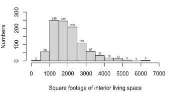
Figure 1: Numbers of interior living space

Figure 1 shows the data distribution, houses with an area of 1000-1500 square footage are the most with 249. There are no houses with space of 5500-6000 square footage. The mean interior living space is 2051.397. The median interior living space is 1900.

Figure 2 describes the construction and design level of the building. Grade is an index from 1 to 13, where 1-3 falls short of building construction and design, 4-6 means below average level, 7 means it has an average level, 8-10 means above-average level, 11-13 means high quality level. According to the Figure 2, it shows that there is no house in a rating of 1-3, 45% of the houses have a rating of 7, and only 2% of the houses have a high-quality level.

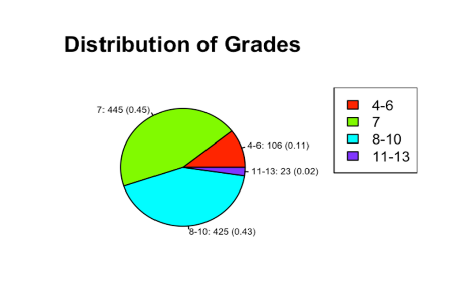
Figure 2: Distribution of Grades

Figure 3 helps readers understand the correlation between the data and the dispersion of the data points. It is worth noting that there is a strong positive correlation between price and the interior living space and grade of houses, which means that as the indoor living area and grade increase, the price also tends to rise. Given these relationships, it is imperative to consider interior living space and grade as influential factors when constructing models of house pricing. Including these variables in the regression models will help to capture the impact of these key factors on price and improve the interpretation of the model based on the data.

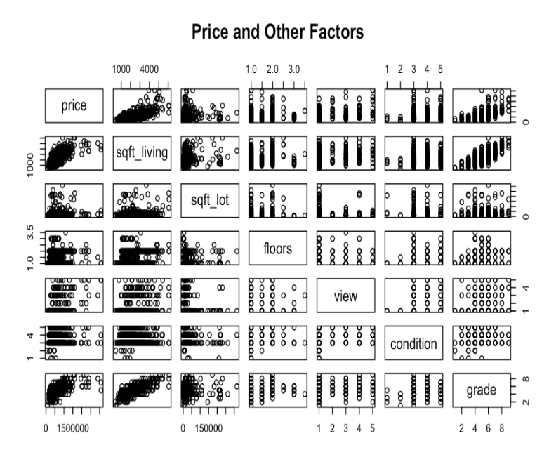
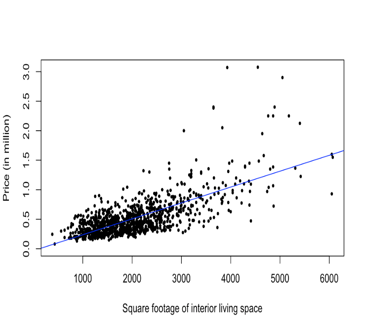
Figure 3: Price and other factors Figure 4: Price and Interior Living Space

Figure 4 is an explanation of the relationship between price and interior space. When interior living space is smaller than 4000, there is a strong linear positive relationship between price and living space. But when the interior living space is larger than 4000, this relationship is less significant. Hence, it is plausible that other factors such as the land space, the condition of houses, and the grade may influence the price. Therefore, a simple linear regression model cannot fully explain the relationship between price and interior living space.

3. Building Models

In this part, the article mainly builds models. By building models to explain the relationship between the variable price and other data, and by training models to predict prices, the article builds three models, multiple linear models, polynomial models, and KNN models. House prices are affected by house structure, plot area, location, etc. At the same time, old and poor quality houses will reduce people’s willingness to buy houses, thereby affecting house sales prices [5, 6]. Therefore, when building the model, the research considers the interior living space, land area, grade (building construction and design), and house view as factors which will affect the price of houses.

3.1. Multiple Linear Regression Model

In order to study and predict house prices, this article introduces multiple linear regression:

\( \text{Y= }\text{β}_{\text{1}}\text{X}_{\text{1}}\text{+}\text{β}_{\text{2}}\text{X}_{\text{2}}\text{+}\text{β}_{\text{3}}\text{X}_{\text{3}}\text{+}\text{β}_{\text{4}}\text{X}_{\text{4}}\text{…+}\text{β}_{\text{0}} \) (1)

In (1), \( \text{β}_{(\text{1,2,3…n})} \) represents the slope coefficient, which represents the change in the dependent variable for each unit change in the corresponding independent variable, and \( \text{β}_{\text{0}} \) is the intercept, which is the bias in machine learning [7]. \( \text{X}_{(\text{1,2,3…n})} \) is the independent variables interior living space, the land space, view, condition, grade.

By training the training set, I get the coefficients and intercept in the model:

\( \text{Price=1.58*}\text{10}^{\text{2}}\text{interiorlivingspace-2.639*}\text{10}^{\text{-3}}\text{landspace+1.158*}\text{10}^{\text{5}}\text{view+3.010*}\text{10}^{\text{4}}\text{condition+8.013*}\text{10}^{\text{4}}\text{grade-5.462*}\text{10}^{\text{5}} \) (2)

3.2. Polynomial Regression Model

After discussing the multiple linear model, the research explores whether there is a nonlinear relationship in the data. The linear regression model assumes that there is a linear relationship between the predictor variable and the response. If the actual data relationship is nonlinear, the prediction accuracy of the model may greatly reduce [8]. Polynomial regression is used to identify nonlinear relationships within the dataset:

\( \text{Y=}\text{β}_{\text{0}}\text{+}\text{β}_{\text{1}}\text{x+}\text{β}_{\text{2}}\text{x}^{\text{2}}\text{+}\text{β}_{\text{3}}\text{x}^{\text{3}}\text{+⋯ +}\text{β}_{\text{n}}\text{x}^{\text{n}}\text{+}\text{β}_{\text{0}} \) (3)

In order to determine the degree in polynomial regression, I use the 5-cross validation method to calculate the root mean square error (RMSE). 5-cross validation is a resampling technique widely used in model selection and evaluation. It prevents overfitting and errors in estimating prediction models [9].

.

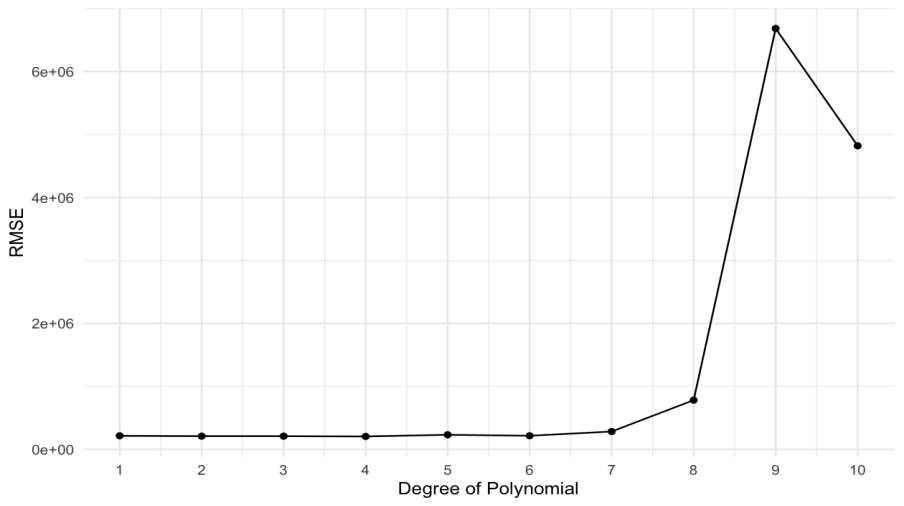
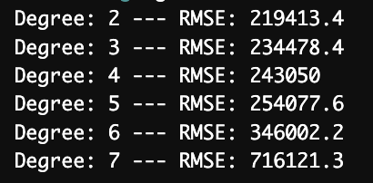
Figure 5 shows that RMSE increases significantly when the degree is greater than 7, indicating that the model performs poorly. As shown in Figure 6, when the order is equal to 2, the RMSE is the smallest. Although the polynomial model with high-order terms can reflect more details in the data, in some cases, the high-order terms will capture noise instead of describing the underlying relationship, resulting in overfitting [10]. When the order is 2, the model can explain the data more effectively. A lower RMSE value indicates that the predictions of models are closer to the actual observed values, which means better accuracy and performance [11]. When the order is set to 2, the model can capture the underlying patterns in the data more effectively than higher or lower orders, which may lead to overfitting or underfitting the data, respectively. Therefore, the polynomial regression model with an order of 2 achieves the best balance:

\( \text{price=1008565+104072*}(\text{interiorlivingspace})\text{+28566*}(\text{interiorlivingspace})^{\text{2}}\text{23981* }(\text{landspace})\text{+2828*}(\text{landspace})^{\text{2}}\text{-27006*}(\text{view})\text{+ 43527*}(\text{view})^{\text{2}}\text{-249362* }(\text{condition})\text{+37864*}(\text{condition})^{\text{2}}\text{-119472*}(\text{grade})\text{+12816*}(\text{grade})^{\text{2}} \) (4)

3.3. K-Nearest Neighbors Model

KNN is a supervised machine learning method that classifies each point by calculating the distance from its k nearest neighbors in the feature space. KNN regression predicts the value of the target variable based on the value of the nearest neighbors.

Euclidean distance is one of the most commonly used distance measurement methods. Using the following formula, it can measure the straight-line distance between a point and another measured point:

\( \text{d}(\text{p,q})\text{=}\sqrt[]{\sum _{\text{i=1}}^{\text{n}} (\text{q}_{\text{i}}\text{-}\text{p}_{\text{i}})^{\text{2}}} \) (5)

Choosing the right k value in KNN is a point that needs to be studied. Different k values may lead to overfitting or underfitting, and lower k values may fluctuate greatly with different data sets. On the contrary, higher k values may not capture the true patterns in the data. The choice of k depends largely on the input data [12].

In building the polynomial model, this paper uses RMSE to evaluate models of different degrees. Similarly, when building the KNN model, it also can be used to determine the appropriate k value by comparing RMSE.

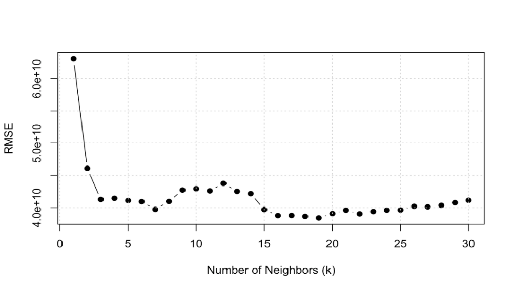
Figure 7: RMSE of different number of neighbors in KNN models

As shown in Figure 7, RMSE is the smallest when k=19, indicating that the KNN model performs best with 19 neighbors. This optimal value allows the model to capture the patterns in the data effectively. Further analysis using a multiple linear regression model including additional variables resulted in an R-squared value of 64.26%, indicating that this multiple linear model can explain more of the data than the linear model. In addition to living spaces, the model also emphasizes the importance of land space, view, condition and grade. The high F-statistic and very low p-value confirm the statistical significance of our model, indicating a strong relationship between the variables and house prices.

While the multiple linear model successfully illustrates the key factors affecting house prices, this paper next builds a polynomial multiple regression model to explain potential nonlinear relationships in the data:

price ~ (sqft_living)^2 + (sqft_lot)^2 + view + condition + grade (6)

By introducing polynomial terms to capture nonlinear effects and provide a more nuanced understanding of the data. Meanwhile the R-square value is increased to 65.14%, which is higher than the R-squares of linear model and multiple linear model. I think the polynomial is the best model of the three models, because it can explain the complexity of the data.

4. Results

After building and training the model, the next step is to test the performance of the model on the test set. The research uses two statistical measures to evaluate the performance of the model, one is R square:

\( \text{R}^{\text{2}}\text{= 1 - }\frac{\text{Residual Variance}}{\text{Total Variance}} \) (7)

The R-squared value ranges from 0 to 1. The larger the R-squared value, the better the model explains the relationship between the dependent variable and the independent variable. Compared with other evaluation parameters, R square is more reliable in regression analysis, so I will use R square as one of the criteria for evaluating the model in this article [13].

Another one is root mean square error (RMSE):

\( \text{RMSE = }\sqrt[]{\frac{\text{1}}{\text{n}}\sum _{\text{i=1}}^{\text{n}} (\text{p}_{\text{i}}\text{-}\text{q}_{\text{i}})^{\text{2}}} \) (8)

Where \( \text{p}_{\text{i}} \) is the actual value, \( \text{q}_{\text{i}} \) is the predicted value, and n is the number of the data. For the case where the estimated error distribution is Gaussian, it is more appropriate to use RMSE to evaluate the model's performance [14].

Table 1: \( \text{R}^{\text{2}} \) , Mean Squared Error and Root Mean Squared Error of the Models

The \( \text{R}^{\text{2}} \) of the multiple linear model is 0.9932, but it has the largest RMSE among the three models, which is \( \text{4.1571*}\text{10}^{\text{5}} \) . In comparison, the \( \text{R}^{\text{2}} \) of the polynomial regression is 0.9986, and it has the smallest RMSE \( \text{1.9092*}\text{10}^{\text{5}} \) . The \( \text{R}^{\text{2}} \) of the KNN model is 0.9985, and the RMSE is \( \text{1.9599*}\text{10}^{\text{5}} \) .

Both the polynomial regression model and the KNN model have better performance in predicting house prices, indicating that the data relationships are not only linear but also involve many nonlinear relationships that the multiple linear model cannot capture.

5. Conclusion

In summary, the analysis of the multivariate linear model, polynomial regression model, and KNN model revealed different patterns in the data. Specifically, the polynomial regression model outperformed the other models, capturing the nonlinear relationship in the data and providing the most accurate predictions. The correlation coefficients in the polynomial regression model show that larger living space and higher building grade generally lead to higher housing prices, while other characteristics such as views and conditions also affect the change of housing prices. This analysis can enhance pricing strategies, strengthen market analysis, and ultimately help buyers, sellers, and developers make more informed decisions. Although the polynomial regression model performed best among the three models, it does not determine that the model is always the best model in all similar datasets. The dataset used is specific to Seattle, Washington. Since housing markets in different regions can vary greatly, the study set in this article does not include important factors such as urban economic indicators, the level of amenities, and the safety of the community, which may limit the accuracy and generalizability of the model. The model may not generalize well to other regions without retraining and adjustment. In addition, regularization techniques such as Lasso or Ridge regression can be used to penalize large coefficients to improve the generalization ability of the model. This study demonstrates the potential of machine learning models in predicting housing prices based on various influencing factors. As technology advances, more research can be conducted using more advanced methods such as neural networks and deep learning to develop more extensive and accurate housing price prediction models.

References

[1]. Hashim, Zainal Abidin. House price and affordability in housing in Malaysia. Akademika 78.1 (2010): 37-46.
[2]. Kadir Atalay, Rebecca Edwards, House prices, housing wealth and financial well-being, Journal of Urban Economics, (2022): 129. https://doi.org/10.1016/j.jue.2022.103438.
[3]. Miu, Peter, and C. Sherman Cheung. Home ownership decision in personal finance: Some empirical evidence. Financial Services Review 24.1 (2015): 51-76.
[4]. El Naqa, I, and, Murphy, M.J. What Is Machine Learning?. In: El Naqa, I., Li, R., Murphy, M. (eds) Machine Learning in Radiation Oncology. Cham: Springer. 2015. https://doi.org/10.1007/978-3-319-18305-3_1
[5]. Wang, L., Wang, G., Yu, H., and Wang, F. Prediction and analysis of residential house price using a flexible spatiotemporal model. Journal of Applied Economics, 25.1(2022): 503–22. https://doi.org/10.1080/15140326.2022.2045466
[6]. X., Cheri. Optimizations of Training Dataset on House Price Estimation, 2nd International Conference on Big Data Economy and Information Management, Sanya, China, 202: 197-203. doi: 10.1109/BDEIM55082.2021.00047.
[7]. Hastie, T., Tibshirani, R., and Friedman, J. The elements of statistical learning: Data mining, inference, and prediction (2nd ed.). Springer, 2009.
[8]. James, G., Witten, D., Hastie, T., Tibshirani, R., and Taylor, J. Linear regression. In An introduction to statistical learning: With applications in python. Cham: Springer International Publishing, 2023: 69-134.
[9]. Berrar, Daniel. Cross-validation. 2nd Edition, Encyclopedia of Bioinformatics and Computational Biology, (2019): 542-545.
[10]. B. Wang, X. Ding and F. -Y. Wang, Determination of polynomial degree in the regression of drug combinations, IEEE/CAA Journal of Automatica Sinica, 4.1(2017): 41-47. doi: 10.1109/JAS.2017.7510319.
[11]. Haiyan, Jiang, Jianzhou, Wang, Jie, Wu, and Wei, Geng. Comparison of numerical methods and metaheuristic optimization algorithms for estimating parameters for wind energy potential assessment in low wind regions, Renewable and Sustainable Energy Reviews, (69)2017: 1199-217. https://doi.org/10.1016/j.rser.2016.11.241.
[12]. Hastie, T., Tibshirani, R., and Friedman, J. The Elements of Statistical Learning: Data Mining, Inference, and Prediction. Springer, 2009.
[13]. Chicco D, Warrens MJ, and Jurman G. The coefficient of determination R-squared is more informative than SMAPE, MAE, MAPE, MSE and RMSE in regression analysis evaluation. PeerJ Computer Science, 7(2021): 623. https://doi.org/10.7717/peerj-cs.623
[14]. Chai, Tianfeng, and Roland R. Draxler. Root mean square error (RMSE) or mean absolute error (MAE). Geoscientific model development discussions, 7.1 (2014): 1525-34.
Cite this article
Zhang,H. (2024). Predicting Housing Prices Using Supervised Machine Learning Models. Advances in Economics, Management and Political Sciences,118,1-7.
Data availability
The datasets used and/or analyzed during the current study will be available from the authors upon reasonable request.
Disclaimer/Publisher's Note
The statements, opinions and data contained in all publications are solely those of the individual author(s) and contributor(s) and not of EWA Publishing and/or the editor(s). EWA Publishing and/or the editor(s) disclaim responsibility for any injury to people or property resulting from any ideas, methods, instructions or products referred to in the content.
About volume
Volume title: Proceedings of the 3rd International Conference on Financial Technology and Business Analysis
© 2024 by the author(s). Licensee EWA Publishing, Oxford, UK. This article is an open access article distributed under the terms and
conditions of the Creative Commons Attribution (CC BY) license. Authors who
publish this series agree to the following terms:
1. Authors retain copyright and grant the series right of first publication with the work simultaneously licensed under a Creative Commons
Attribution License that allows others to share the work with an acknowledgment of the work's authorship and initial publication in this
series.
2. Authors are able to enter into separate, additional contractual arrangements for the non-exclusive distribution of the series's published
version of the work (e.g., post it to an institutional repository or publish it in a book), with an acknowledgment of its initial
publication in this series.
3. Authors are permitted and encouraged to post their work online (e.g., in institutional repositories or on their website) prior to and
during the submission process, as it can lead to productive exchanges, as well as earlier and greater citation of published work (See
Open access policy for details).