


1. Introduction
In the rapidly evolving global economy and technological landscape, the energy challenge is a universal concern. Energy is a fundamental driver of societal progress, and its absence would hinder development. With profound implications for all aspects of human life and production, energy is a linchpin for each country's political and economic security[1], directly influencing future development and survival.
As an important part of energy, electric energy plays a key role in every country and plays an irreplaceable role in ensuring industrial and agricultural production, military defense and people's livelihood. Therefore, we need to deeply understand the current situation of electricity consumption, and make a scientific prediction of power consumption, then explore the causes of power consumption changes and finally take targeted scientific measures. Only in this way can we achieve the sustainable development of electric energy, which is of great significance to the sustainable development of the country and the economy.
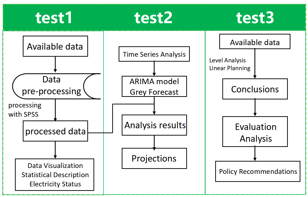
In this paper, the available data is preprocessed by spss software, and appropriate methods are selected to fill in the missing values and deal with the outliers. Then, the processed data are used to forecast and analyze the power generation and total power consumption of different energy sources at different resolutions based on seasonal ARIMA model and grey prediction model. Finally, the evaluation system and optimization model of energy allocation strategy are established based on REAO model, and the policy recommendations are given according to the final conclusions.
To avoid complex descriptions and to visualize our work process, the flow chart is shown in Figure 1.
2. Time Series Models
2.1. Data pre-processing
We utilize Coordinated Universal Time (UTC) as the standard and exclude European Union time. Additionally, we simplify the time format.
(1) Initially, columns with missing values exceeding 50% were eliminated. The abundance of missing data made reasonable filling impractical.
(2) Regarding the data columns "BE_wind_offshore_generation_actual," "BE_wind_onshore_generation_actual," and "BE_wind_generation_actual," wherein the total wind production electricity equals land wind production electricity plus offshore wind production electricity, a triadic relationship is established among these three columns.
(3) Data columns with minimal missing values underwent weighted average imputation based on the temporal proximity, utilizing both periodic and before-and-after weighted mean methods.
(4) Data columns with a higher prevalence of missing values were treated using the periodic and linear interpolation method to fill in values aligned with the overall trend.
(5) Addressing anomalous data, such as the "price_day_ahead" column with negative data column weights, necessitates correction. For other conspicuous anomalies, the regression interpolation method was applied.
2.2. Analysis Results Presentation
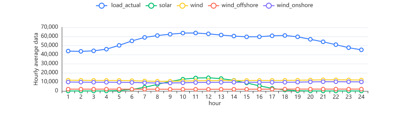
Based on the processed data, the mean values of the hourly, monthly and yearly data are calculated to analyze this question. The graph is shown below[2].
Figure 2: Hourly data averages. |
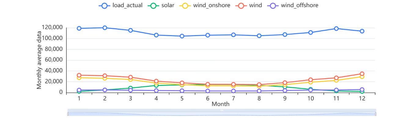
Figure 3: Daily data averages. |
Figure 4: Average volume of data per year. |
Figure 5: Average amount of capacity per year. |
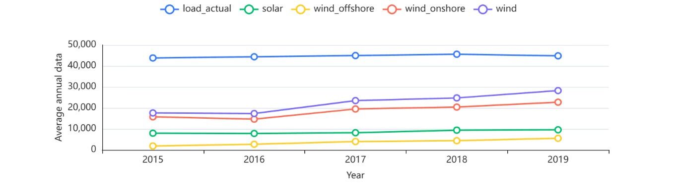
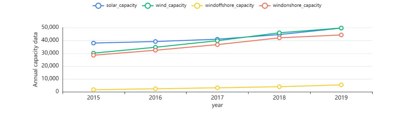
Regarding the average value of each year's data, the 2020 data was discarded because it only goes up to September and the size of the data will change with the month, which will result in errors in calculating the average value.
2.3. Analyzing Time Series Models for Energy Consumption
We primarily employ time series analysis, utilizing the ARIMA model[3] and gray scale forecasting, to address the issue at hand.
In the context of wind power generation time series, we decompose the data into trend, seasonal, and stochastic components to preliminarily ascertain the seasonal effects. The significance p-value is 0.000***, indicating significance at the specified level and leading to the rejection of the original hypothesis that the series is a smooth time series.
For the variable wind_generation_actual, analysis of the residual Q statistic yields the following insights: Q6 lacks significance at the specified level, indicating that the hypothesis of residuals conforming to a white noise series cannot be rejected, and the model generally meets the requirements. However, the goodness-of-fit R² of the model is 0.414, signifying suboptimal performance.
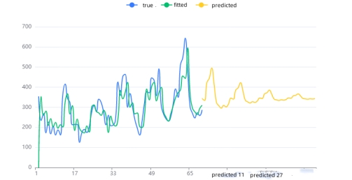
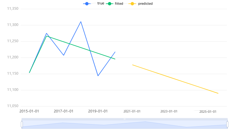
The ensuing figure depicts the raw data plot, model-fitted values, and model-predicted values for this time series model.
Figure 6: Time series chart of wind energy generation. |
Figure 7: Time series chart of wind energy generation. |
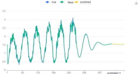
For the solar power time series, the analytical approach aligns with the previous subsection. Focusing on the variable solar_generation_actual, the Q statistic analysis reveals that Q6 lacks significance at the specified level. The hypothesis that the residuals of the model conform to a white noise series cannot be rejected. Additionally, the model's goodness of fit, R², stands at 0.935, signifying excellent performance and general adherence to requirements.
In the context of solar_generation_actual, the system automatically determines optimal parameters through the AIC information criterion. The resulting ARIMA model (1,1,2)[4] is applied to 1-differenced data, yielding the following model equation
\( y(t)=6.754+0.445y(t-1)-0.649ε(t-1)-0.157ε(t-2) \) (1)
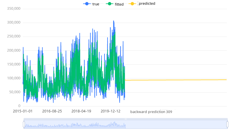
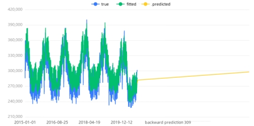
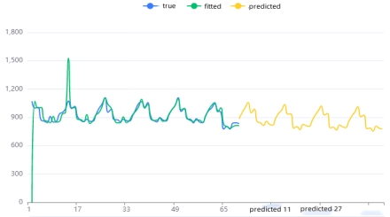
For the power consumption time series, the system automatically identifies optimal parameters using the AIC information criterion. The resulting ARIMA model (2,1,1) is applied to the variable load_actual_entsoe_transparency. The analysis of the Q statistic reveals that Q6 lacks significance at the specified level, and the hypothesis that the residuals conform to a white noise series cannot be rejected. The model's goodness-of-fit, R², stands at 0.735, indicating satisfactory performance that essentially meets the requirements.
The ensuing figure illustrates the raw data plot, model-fitted values, and model-predicted values for this time series model.
Figure 8: Electricity consumption time series chart. |
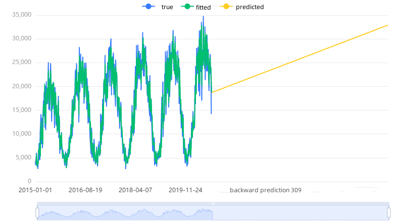
Figure 9: Time series chart of wind energy generation. |
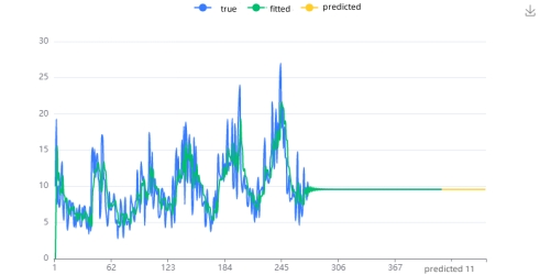
For wind power generation time series, the same ARIMA model was used.The analysis reveals a stable time series for wind power with a suboptimal model performance (R² = 0.401). Conversely, solar power exhibits a smooth time series with a well-performing model (R² = 0.918). Visualizations depict the original data, model fitted values, and predictions for each respective time series.
Figure 10: Time series graph of solar power. |
Figure 11: Electricity consumption time series chart. |
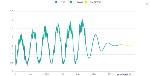
The power consumption time series exhibits a smooth pattern with a well-performing model (R² = 0.831), while the wind power generation time series displays a smooth pattern with suboptimal model performance (R² = 0.414). Visualizations depict the original data, model fitted values, and predictions for each respective time series.
Figure 12: Time series chart of wind energy generation. |
Figure 13: Time series graph of solar power. |
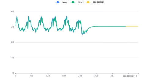
The solar power time series exhibits a smooth pattern, but the model's performance is suboptimal with an R² of 0.496. In contrast, the power consumption time series also demonstrates a smooth pattern, but the model performs poorly, with an unusually high R² of 2.115. Visualizations depict the original data, model fitted values, and predictions for each respective time series.
Figure 14: Electricity consumption time series chart. |
Figure 15: Fitted prediction graph of gray prediction model. |
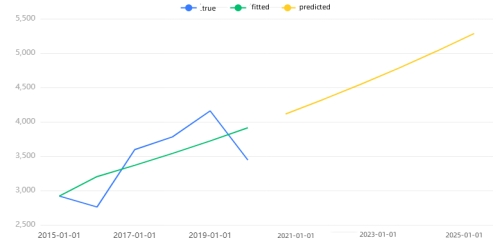
For wind power generation, the application of the gray prediction GM (1, 1) model proves effective in handling limited annual data, yielding a qualified model with a posterior difference ratio of 0.516 and an average relative error of 8.823%. Similarly, for solar power and power consumption time series, the same model exhibits high accuracy with posterior difference ratios of 0.246 and 0.623, and average relative errors of 3.607% and 0.33%, respectively. Visualizations depict the fitted prediction graphs for each time series.
Figure 16: Fitted prediction graph of gray prediction model. |
3. Strategic Evaluation and Optimization Framework for Renewable Energy Allocation
Firstly, based on the hierarchical analysis (AHP)[5], a comprehensive evaluation module is built to set core indicators from four aspects: electric energy, economy, environment, and cost, and start to subdivide them level by level to establish a hierarchical structure and generate a judgment matrix with affiliation scale. Second, based on the comprehensive evaluation results and linear programming model, the optimization module is constructed to optimize the allocation of quota weights for development.The structure diagram is shown below.
Figure 17: REAO Model Framework. |
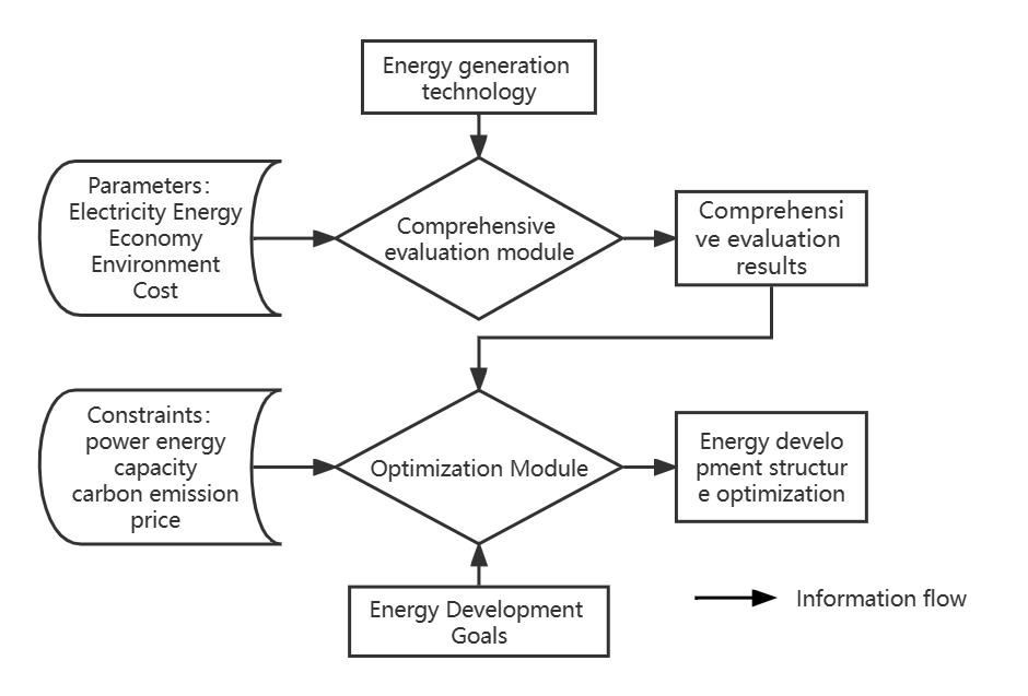
We establish a systematic link among influencing factors, categorizing indicators into quantitative and qualitative aspects. Thermal power, hydropower, nuclear power, wind power, and solar power generation serve as evaluation objects. Indicators, including actual electricity generation, economic considerations based on energy reserves and distribution characteristics, environmental impact metrics like carbon emissions, and cost indicators, are analyzed using a qualitative and quantitative approach. Data standardization employs the efficacy coefficient method to reflect the relative merits of each indicator in the series.
We take the maximization of the combined evaluation score portfolio as the objective function, and add four constraints of electric energy, capacity, carbon emission and price to maximize the combined benefits of the renewable energy portfolio to establish a linear programming portfolio.
The following table shows the judgment matrix constructed.
Table 1: Weight judgment matrix.
Indicators | power energy | economy | environment | cost |
power energy | 1 | 5/4 | 3/4 | 4/3 |
economy | 4/5 | 1 | 2/3 | 4/5 |
environment | 4/3 | 3/2 | 1 | 3/2 |
cost | 3/4 | 5/4 | 2/3 | 1 |
The weight calculation result of hierarchical analysis showed that the weight of power energy was 25.975%, the weight of economy was 19.854%, the weight of environment was 32.33%, and the weight of cost was 21.842%. Moreover, the maximum characteristic root is 4.011, and the corresponding RI value is 0.882 according to the RI table, so CR=CI/RI=0.004<0.1, which passes the one-time test.
The index assignment, data standardization and comprehensive evaluation results are shown in the following table. It can be seen that, considering the four dimensions of electricity, economy, cost, and environment, the five energy utilization indices are, from highest to lowest, nuclear power, hydro power, solar power, wind power, and thermal power. This is consistent with the results of relevant studies done by the Chinese Academy of Sciences and the National Development and Reform Commission (hydropower is first, wind is second), but slightly different from the results of international studies (wind is more sustainable than hydropower), the reason being that China's nuclear and hydropower development time and cost and technology maturity advantages are much higher than other energy sources, given the small difference in resource endowment and environmental impact.
Table 2: Comprehensive index assignment.
Energy | Electricity Generation (billion kilowatts) | Reserves (qualitative) | Distribution Characteristic (qualitative) | Carbonemission (g/kwh) | Powergeneration Cost (yuan/kwh) | |
Thermal Power | 28200 | 3 | 7 | 975.3 | 0.29 | |
Utilities | 4826 | 7 | 5 | 25.707 | 0.1 | |
Nuclear Power | 1950 | 7 | 6 | 11.9 | 0.22 | |
Wind Power | 2819 | 8 | 7 | 13.53 | 0.34 | |
Solar Power | 858 | 9 | 10 | 62.5086 | 0.44 | |
Table 3: Comprehensive evaluation results.
Energy | Electricity | Economy | Environment | Cost | Overall Score |
Thermal Power | 10 | 4.2 | 6 | 7.76471 | 7.0670 |
Utilities | 6.5805 | 6.4 | 9.94267 | 10 | 8.5432 |
Nuclear Power | 6.59754 | 6.7 | 10 | 8.58824 | 8.6253 |
Wind Power | 6.86885 | 7.7 | 9.99323 | 7.1764 | 8.1321 |
Solar Power | 6 | 9.3 | 9.78988 | 6 | 8.2882 |
Weights | 0.2598 | 0.1985 | 0.3233 | 0.2184 |
The evaluation module gives comprehensive evaluation results based on a series of core indicators, but in actual policy formulation, it is necessary not only to optimize various energy development structures under the premise of meeting the energy demand for sustainable economic development, but also to consider a series of objective constraints faced in actual energy development. In this section, based on the evaluation, the optimization module is further applied to optimize the development scenarios of different energy sources.
Specific constraints explained:
(1) The weight of each energy source is greater than or equal to 0.
(2) The sum of the weights of the five energy sources is equal to 1.
(3) Cost constraint: the development of energy sources must bring cost improvement, and the future average cost of optimized energy sources is less than or equal to the existing average cost.
(4) Carbon emission constraint: make the future total energy CO2 emissions above the average level of the current 5 energy sources CO2 emissions.
(5) Economic constraint: the future economic development of the optimized energy source is above the average level of the current economic development of the five energy sources.
(6) Electric energy constraint: the electric energy production of the optimized energy source is above the average level of the electric energy production of the current five energy sources.
Substituting the data, the following system of equations is obtained:
\( max z =7.067×{X_{1}}+8.5432×{X_{2}}+8.6253×{X_{3}}+8.1321×{X_{4}}+8.2883×{X_{5}} \) S.t. \( \begin{cases} \begin{array}{c} {X_{1}}+{X_{2}}+{X_{3}}+{X_{4}}{+X_{5}}=1 \\ {X_{1}} \gt 0;{X_{2}} \gt 0;{X_{3}} \gt 0;{X_{4}} \gt 0;{X_{5}} \gt 0 \\ 10{X_{1}}+{6.58X_{2}}+6.598{X_{3}}+6.869{X_{4}}+6{X_{5}}≥7.209 \\ 4.2{X_{1}}+{6.4X_{2}}+6.7{X_{3}}+7.7{X_{4}}+9.3{X_{5}}≥6.86 \\ 6{X_{1}}+{9.943X_{2}}+10{X_{3}}+9.993{X_{4}}+9.79{X_{5}}≥9.145 \\ 7..765{X_{1}}+{10X_{2}}+8.588{X_{3}}+7.176{X_{4}}+6{X_{5}}≥7.906 \end{array} \end{cases} \) | (2) |
z denotes the objective function to optimize the comprehensive evaluation score, X1~X5 denote the energy share of thermal, hydro, nuclear, wind and solar power respectively.
The optimal weights for the five renewable energy sources can be obtained by solving the linear programming as shown in the table below.
Table 4: Weighting ratio optimization results.
Parameters | Solve for the value |
z(Target value) | 8.132 |
X1(Thermal power) | 0.137 |
X2(Hydropower) | 0.142 |
X3(Nuclear Power) | 0.176 |
X4(Wind Power) | 0.545 |
X5(Solar Power) | 0 |
4. Conclusions and Recommendations
We have developed a comprehensive model for evaluating and optimizing the structure of China's energy sources. This model encompasses four key dimensions: economic, cost, electric energy, and environmental considerations. We have analyzed the current status of each evaluation criterion and systematically assessed the five major energy sources. The findings indicate that both nuclear power and hydropower rank highly. Utilizing the evaluation results, we applied a linear programming model to simulate and optimize the future energy development structure. This optimization considered constraints related to cost, energy, capacity, and carbon emissions. The results reveal that thermal power, hydro power, nuclear power, wind power, and solar power contribute 13.7%, 14.2%, 17.6%, 54.5%, and 0% of the quota, respectively.
Drawing on the comprehensive evaluation and optimization outcomes, we propose the following recommendations for promoting sustainable electric energy development:
(1) Harnessing Wind and Solar Energy:Wind and solar energy exhibit significant development potential. We advocate for a sustained interest analysis, emphasizing the vigorous development of wind energy. Furthermore, enhancing the conversion efficiency of solar energy through increased support for technological research and development within the solar industry is crucial. To foster a more extensive domestic market in China, it is imperative to establish clear resource development goals and implement initiatives supporting the solar energy industry.
(2) Establishment of Power and Energy Development Plans:The Chinese government should formulate overarching sustainable development goals that integrate economic and environmental planning. Collaborating with various departments, the power industry, and the public, the government should set binding targets for power energy development. Implementing comprehensive measurement, supervision, and assessment measures is essential. Government departments at all levels should establish an information-sharing platform to monitor power companies' real-time carbon emissions and conduct regular assessments.
(3) Reform of the Electricity Tariff System:China's electricity tariff mechanism, particularly in the pricing of new energy tariffs, is imperfect. The government should persist in deepening the reform of the electricity tariff system to establish a rational mechanism that aligns with market supply and demand while considering resource and environmental costs.
References
[1]. Cable, Vincent. "What is international economic security?." International Affairs 71.2 (1995): 305-324.
[2]. Scientific Platform Serving for Statistics Professional 2021. SPSSPRO. (Version 1.0.11)[Online Application Software]. Retrieved from https://www.spsspro.com.
[3]. Shumway, Robert H., et al. "ARIMA models." Time series analysis and its applications: with R examples (2017): 75-163.
[4]. Xue, Dong-mei, and Zhi-qiang Hua. "ARIMA based time series forecasting model." Recent Advances in Electrical & Electronic Engineering (Formerly Recent Patents on Electrical & Electronic Engineering) 9.2 (2016): 93-98.
[5]. Yang, Xiaojun, Liaoliao Yan, and Luan Zeng. "How to handle uncertainties in AHP: The Cloud Delphi hierarchical analysis." Information Sciences 222 (2013): 384-404.
Cite this article
Sang,M. (2024). A Study on Energy Production and Consumption Based on Seasonal ARIMA and REAO. Advances in Economics, Management and Political Sciences,112,47-56.
Data availability
The datasets used and/or analyzed during the current study will be available from the authors upon reasonable request.
Disclaimer/Publisher's Note
The statements, opinions and data contained in all publications are solely those of the individual author(s) and contributor(s) and not of EWA Publishing and/or the editor(s). EWA Publishing and/or the editor(s) disclaim responsibility for any injury to people or property resulting from any ideas, methods, instructions or products referred to in the content.
About volume
Volume title: Proceedings of the 8th International Conference on Economic Management and Green Development
© 2024 by the author(s). Licensee EWA Publishing, Oxford, UK. This article is an open access article distributed under the terms and
conditions of the Creative Commons Attribution (CC BY) license. Authors who
publish this series agree to the following terms:
1. Authors retain copyright and grant the series right of first publication with the work simultaneously licensed under a Creative Commons
Attribution License that allows others to share the work with an acknowledgment of the work's authorship and initial publication in this
series.
2. Authors are able to enter into separate, additional contractual arrangements for the non-exclusive distribution of the series's published
version of the work (e.g., post it to an institutional repository or publish it in a book), with an acknowledgment of its initial
publication in this series.
3. Authors are permitted and encouraged to post their work online (e.g., in institutional repositories or on their website) prior to and
during the submission process, as it can lead to productive exchanges, as well as earlier and greater citation of published work (See
Open access policy for details).
References
[1]. Cable, Vincent. "What is international economic security?." International Affairs 71.2 (1995): 305-324.
[2]. Scientific Platform Serving for Statistics Professional 2021. SPSSPRO. (Version 1.0.11)[Online Application Software]. Retrieved from https://www.spsspro.com.
[3]. Shumway, Robert H., et al. "ARIMA models." Time series analysis and its applications: with R examples (2017): 75-163.
[4]. Xue, Dong-mei, and Zhi-qiang Hua. "ARIMA based time series forecasting model." Recent Advances in Electrical & Electronic Engineering (Formerly Recent Patents on Electrical & Electronic Engineering) 9.2 (2016): 93-98.
[5]. Yang, Xiaojun, Liaoliao Yan, and Luan Zeng. "How to handle uncertainties in AHP: The Cloud Delphi hierarchical analysis." Information Sciences 222 (2013): 384-404.