1. Introduction

This paper analyzed the factors that affect housing prices in Beijing. Nowadays, mainly attributing to increasing modernization and economic breakthrough, the housing prices surges in especially large cities in China. Although current researches have revealed significant insight toward the factors that affect the property values in Beijing or other China’s large cities, there are few that only used quantitative data, and also that most of them are using relatively old data, which limits their predictability of constantly changing housing prices. This paper aimed to study the factors that affect Beijing’s housing prices solely using quantitative data from an econometric scope, allowing for more subjective and data-based statistical analysis. The research is significant on its usage of regression analysis and quantitative data, as well as the dataset obtained from the period in which Beijing’s undulation and movements in housing prices are relatively large. The large data size also contribute to a relatively accurate estimate.

Fang et al. conducted a large-scale investigation based on dataset from China Commercial Bank about mortgage loan from 2003 to 2013, using hedonic price regressions [1]. The research reveals the price surge was especially significant in first-tier cities (Beijing, Shanghai, Shenzhen, and Guangzhou) with an average annual growth rate of 13.1%; the growth rate was also high in second and third tier cities, with growth rates of 10.5% and 7.9% respectively. This rapid growth is even higher than the US housing bubble and was comparable to Japan’s bubble in the 1980s; yet, the downpayment required for the Chinese mortgage is 30%, which was significantly higher than that in the US or in Japan, preventing subprime crisis. On the other side, the real household disposable income has risen 9%, buffering against potential housing bubble collapse.

Next, Gleaser et al. have shown that the demand for buying houses is mainly rooting from people in middle-aged with sufficient savings or income [2]. Owning a property in a first-tier city can also represent a premium or a higher status. People buying houses have different motivations like as a heritage for children, as an investment, as a show-off of wealth, or as a speculation; the incentives for the demand side varies but has Chinese unique features. On the other hand, the supply of Chinese housing is relatively elastic, inferring from the high vacancy rate of houses and continuing casting and constructions of new housings. The Chinese government is trying to limit supply, not through restricting the number of housings build, but by raising the interest rate and minimum down payment, making those with high-enough income or saving can buy houses. This tendency of encouraging construction but restricting people from getting loans to buy is an opposite choice from the US government’s act.

When comparing with other countries, a good comparison subject would be Japan, as China and Japan are both economically developed countries in Asia. The statistical experiment published in 2006 by Shimizu et al. examined the temporal divergence between actual transaction prices and appraised land prices, such as official land prices [3]. In the bubble period in Japan during 1990s, appraised land prices were only about 50-60% of the actual market prices. However, after the bubble burst, the appraised prices were approximately 20% higher than market prices. They pointed out that price evaluation and prediction models are not the problem; rather, the speed that is overly high to obtain information and the choice of the technology to use to was responsible.

On the other hand, considering price from air pollution aspect, Wenhao et al. have pointed out that “For every 1% increase in annual mean PM2.5 concentration, house prices decrease by 0.541%”; yet, when educational facilities and disposable income. The results of the regression using instrumental variables show that when per capita disposable income is less than CNY 101,185, house prices will decrease by 0.425% for every 1% increase in PM2.5; otherwise, house prices will decrease by 0.460% for every 1% increase in PM2.5 [4].

Additionally, research done by Shi et al. studied the ten communities in Beijing with highest housing prices and the ten communities with lowest prices; without using statistical tools solely relying on the qualitative characteristics of the housing units, the study shows that Haidian, Dongcheng, and Chaoyang are the regions with the highest housing prices, and the lowest one tend to locate in economically underdeveloped areas [5]. It also noted that political factors and social factors (i.e. Immigration and Birth Rate) all contributes intricately in addition to economic factors. Simply saying economic condition of the region, it not only accounts for economic growth, but also the mutually effecting role that high average income in one region leads to higher ability of consumption which indicates better willingness to pay for higher housing prices.

From another viewpoint, paper by Zhou et al. investigated how access to public transportation is also a contributing factor to the property values, when considering whether Beijing is a monocentric or a polycentric city [6]. The research revealed that in addition to the difference of eastern and western part within Beijing, whether the part is suburban or urban, whether the region is close subcenters. In suburban areas, there are few metro and bus stations, so having more subway lines near the house significantly improves access, which makes the number of public transportation having a larger impact on suburban-area houses’ prices than the impact on urban areas. It is also noticeable that Beijing has already have twenty metro lines and over one thousand bus routes at the time of 2020.

Lastly, mixed usage of Beijing’s land was investigated by Yang et al., indicating that mixed use of land - in other words, buying lands not only for living but also for other factors including speculation - correlated positively with the land prices [7]. While the paper only studied second-hand houses, it drew conclusions that if more possible rent can be earned from lending the houses, the investment toward real estate will largely increase, driving up the value of property rights. This speculative demand also adds up to the complicated mechanisms in the Beijing housing price markets. Also, when compared with Japan where there was similar situation during bubble, the demand for houses in China is much larger, since Japan is facing decreasing demand for space or land due to declining birthrate and aging population, according to Shimizu’s research in 2014 [8].

2. Methodology

2.1. Data Source

The dataset was from Kaggle in csv format, and the original data was from the website of Lianjia. It contains the housing prices and other factors about the houses in Beijing. Since the dataset contained a large amount of data (318851 unique values), the large size of data was not suitable for analysis. In order to ensure the estimate is accurate while doing the regression compactly, I have used the first 3139 data with not nan values. The data from Lianjia is well-documented, and thus reliable, considering its well-known status in Chinese property agencies.

2.2. Variable Selection

The original dataset contained some nan data, which is not suitable for analysis. Therefore, this paper only used the variables with no missing data to conduct regressions. Price is chosen as the dependent variable since what people want to know is how other factors are impact on the housing prices or not. Based on analysis on which factors is likely contributing, following variables are chosen as independent variables (Table 1).

Table 1: Variables Used in the OLS Regression

2.3. Method Introduction

Initially, Ordinary Least Square regression of multiple variables weas conducted. VIF test was used to investigate whether there is multicollinearity or not. Residual test was used to test if the residual mean equals zero or not. White test was used to test whether or not there is heteroskedasticity in the OLS regression.

\( y={β_{0}}+{β_{1}}{x_{1}}+{β_{2}}{x_{2}}+{β_{3}}{x_{3}}+{β_{4}}{x_{4}}+{β_{5}}{x_{5}}+{β_{6}}{x_{6}}+{β_{7}}{x_{7}}+ε \) (1)

However, to address potential possibility of endogeneity issue, Two-Stage Least Squares (2SLS) Regression Analysis is applied.

\( y={β_{0}}+{β_{1}}･ E({x_{1}})+{β_{2}}{x_{2}}+{β_{3}}{x_{3}}+{β_{4}}{x_{4}}+{β_{5}}{x_{5}}+{β_{6}}{x_{6}}+{β_{7}}{x_{7}}+ε \) (2)

3. Results and Discussion

3.1. Results of the OLS Regression

Table 2 shows the results of the OLS Regression. The p-values for all of the coefficients are less than 0.05, and none of the 95% confidence interval contains 0; both facts indicate that all of the listed independent variable have statistically significant correlation with the independent variable - price. The coefficient of square is negative meaning that as the total housing area of a typical home increases, the price will decrease, which is apparent regardless of other factors. Other variables’ coefficients are all positive. The coefficient for ladderRatio is especially large (as ladderRatio increase by one unit, price will increase 2716.725), followed by drawingRoom and subway.

Table 2: OLS Regression Results

As shown in Table 3, the p-value associated with F-statistic is 0.00, suggesting that there is convincing evidence against the null hypothesis that all coefficients are zero. In other words, overall F-test for the model is highly significant and the model is significant. Table 3 also shows that the R-squared value is 0.8689. This means that 86.89% of the variation in price (dependent variable) can be explained by variation in the independent variables, validating the fitness of the regression.

Table 3: Other Statistics Associated with the OLS Regression

Subsequently, to test whether the independent variables have high correlation with one another, VIF test is applicated. The results (Table 4) show that all of the VIF are less than 5. This means that there is multicollinearity issue but it is not serious. Additionally, since the mean VIF is close to 1, it can be concluded that multicollinearity is very mild.

Table 4: Results for the VIF Test

Next, to test if the linear regression model fits in the correlation between variables, residual plot is made. As shown in Figure 1, the plot showed mild pattern.

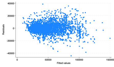
Figure 1: Residual Plot

Therefore, residual test (one sample t-test) with “the mean of the residuals is zero” as the null hypothesis is conducted. The p-value of 1.00 foretells that there is no convincing evidence that the residual mean is different from zero. Since the errors are centered around zero, the regression model is fit on average in terms of residual behaviors.

3.2. Robust Regression Results

To test heteroskedasticity and avoid unreliable estimates, the White test was conducted. The Chi-square test statistic value is 422.70, degree of freedom is 33, and the p-value is 0.0000, confirming the presence of heteroskedasticity. To address heteroskedasticity issue and better promote accuracy of the estimate, the subsequent regressions will use robust standard errors.

Adjusted to the robust standard errors, p-value for the livingRoom coefficient increased to 0.063 (0.063<0.05). Yet, it is lower than the significance level of 0.1, so the effect of number of living rooms on the house’s price still can be said significant (Table 5).

Table 5: OLS Regression with Robust Standard Errors

3.3. Endogeneity Issue

Although the regression has overall high fitness on the estimate, there is another concern: endogeneity. The conventional one-step OLS regression may render endogeneity issue considering theoretical contexts. It can be alleviated by using a 2SLS; when Ou et al. is studying about how PM2.5 levels play a role on urban cities’ housing prices, suggesting its usefulness in analyzing housing prices determining factors [9]. The variable square may be correlated with error term, resulting in such an issue. Firstly, simultaneity may exist. The size of the house may influence the price, and vice versa - higher prices may be a incentives for developers to build larger houses, seeking for the expected higher selling prices. Such an mutual influence can make the variable square and error term correlated, inducing endogeneity issue. Secondly, there may be omitted variable bias. Square could be correlated with unobserved factors such as neighborhood quality or demand fluctuations, proximity to amenities, or school districts. The study by Shi et al. have pointed out that the choice of the size of the house to live in should vary largely, depending on the buyer’s income level and social background [5]. Putting this into mind, the size of the house that a family wants to live in is definitely larger than that of a young person living alone (square is larger). Economic conditions of people with families are definitely better than those of freshmen, fore instance. Thus, they can afford higher price. This mutually effecting relationship, in other words, reverse causation, precludes us from drawing causal relationship between price and the variables, especially square. The housing prices-to-income ratios are calculated by Fang et al. [1]. In the sampled Chinese cities, price-to-income ratio is in the range of 6 to 10. In 2016, the price of a house with 90 square meters in Shanghai or Beijing is 25 times the average income of households [2].

Based on the viewpoint of this ratio, since people living in larger houses tend to hold families and thus a higher disposable income than freshmen. This makes the payment for buying houses occupy a smaller portion of the disposable funds for those holding families than the young; thus, their demand for buying the house is more elastic. When taking into account the economic conditions of the people who have demand for this house and the elasticities for their demand, it is possible that those omitted variables positively influencing housing prices, rather than square directly causing the price increase. The study also reveals that most Chinese buyer of houses are middle-aged people or above, largely attributing to their more stable savings than youngers. The motivations for them to purchase houses includes to use real estate as an investment or saving for retirement, or for their children’s marriage. The few chances of investment and expected relatively low returns of investment on finance products are driving people with abundant income or saving to devote their money into buying houses (Table 6).

Table 6. Possible Choices for Instrumental Variable

Yet, 2SLS using Cid as an instrument variable (IV) yields multicollinearity issue, so it is not suitable as an IV. This may be because the ID number in some way is correlated with other variables. Also, when kitchen is used as an IV for square, the p-values for all regressors are larger than any possible significance level. This makes the correlation not statistically significant, so using kitchen as an IV for square is not suitable. Other variables alone were not suitable as well, either because it disqualifies the correlation between independent variables and dependent variable or because the endogeneity test had a small p-value. Thus, several variables need to be combined as IVs for square.

3.4. Results of the 2SLS Regression

The results of the 2SLS regression using bathroom and follower as IVs is shown in Table 7. The p-values for square, drawingRoom, ladderRatio, subway, communityAverage are less than 0.05, suggesting there is statistically significant correlation between these variables and price. Coefficient of square is -52.274343. This indicates that for each additional one unit of square meter of the house, the price will decrease by 52 units; in other words, larger houses tend to have slightly higher prices than smaller ones. It can be inferred that Beijing’s dwellers have larger demand on smaller housings. The coefficient for subway is positive and is relatively large (974.9528), which every small improvement in access to subway station is associated by a relatively large increase in price. This supports what is argued in other papers that the access to subway or other transportation including buses indeed is a contributing factor in determining the house’s price. Positive coefficient for communityAverage indicate that the overall reputation or price level of the community significantly affects the price of individual properties. This reflects a broader trend in Beijing, where buyers are willing to pay a premium for homes in well-established or prestigious communities, particularly those with better amenities or a higher social status. This trend ties into the broader socio-economic context of Beijing, where the rapid growth of wealth and urban development drives demand for properties in prestigious neighborhoods.

Table 7: 2SLS Regression with Robust Standard Errors

As shown in Table 8, the Chi-square statistic of 14163.62 as well as the p-value smaller than any possible significance level indicate that the model has an overall statistically significance. In other words, the independent variables collectively are able to explain the variation in the dependent variable (price), since the null hypothesis (H0: None of the independent variables in the model explain the dependent variable) fails to be rejected. Also, the R-squared value of 0.8688 means that 86.88% of the change in \( y \) (price) can be explained by the independent variables, suggesting the variables are suitable predictors.

Table 8: Other Statistics Associated with the OLS Regression

Lastly, the endogeneity test (results shown in Table 9) yields p-values that fail to rejects the hull hypothesis (H0: Variables are exogenous). There is no convincing evidence that the variables are endogenous. Thus, endogeneity issue is effectively alleviated by using bathroom and followers as IVs for square.

Table 9: The Results for Endogeneity Test

3.5. Discussion

By VIF test, White test, residual test, and endogeneity test, the potential issues of the model is detected and addressed to persue a more accurate estimates. With this in mind, some implications can be drawn.

Primarily, the negative coefficient between square and price can be analyzed. This can be due to the inability for people - especially the younger generation who do not need very large houses to afford the overly high housing prices in Beijing, but have demand to live in Beijing; preference for smaller, more centrally located properties or a saturation effect where bigger properties reduce marginal price per square meter can be seen. This trend significantly differs from Japan, which tend to have similar character as China (Tokyo as the main center with most population centered at, and both countries are large economic forces in Asia). According to Inoue et al., factors like geographic segmentation and local neighborhood characteristics is the determinant factor in Tokyo; also, in Tokyo, properties in Minato-city and Shibuya-city retain high per-square-meter prices especially for larger homes [10]. This can be attribute to people living in the expensive area in Tokyo is living there from economic booth period, so they already have wealth and holds families and thus prioritize larger living spaces in premium locations. By contrast, in Beijing, access to amenities such as subway stations dominate buyer preferences, possibly due to people living there is still workers and do not have sufficient funds to support families and larger housings, but only have the need to stick in the economic center, Beijing.

When considering the fitness of IVs, the reason why variable bathroom is suitable as an IV for square can be because it decently satisfies the two conditions: relevance and exclusion. The number of bathrooms is usually determined when the house is designed based on the size of the house and the expected living needs, so it is related to the square footage of the house (relevance) and will not change due to other fluctuations - namely, will not change following error term (exclusion). On explanation for why kitchen cannot be a suitable IV but bathroom can when combined with the variable follower as IVs, is that the number of kitchen can be measured of the degree of gorgeousness of the house. In other words, it can correlated with omitted variables like how lavish the furnishing is. This do not fully meet its exclusion condition with the error terms, so disqualifies kitchen as an IV to solve endogeneity issue. Although kitchens can be decorated or ornamented in a fancy way that may affect prices, bathroom cannot indicate the degree of fancy of the house, so cannot correlated with error terms to effect housing prices. Subsequently, while DOM was not effective, followers was more relevant, as shown by a larger F-statistic when followers was used as an IV. However, the use of followers alone did not completely solve the endogeneity issue, as indicated by a small p -value in the endogeneity test. A combination of bathroom and followers as IVs for square served to successfully solve endogeneity issue in the model. This is evident in following results. Firstly, the coefficient of square yields a p-value of 0.000, indicating with the usage of the IVs, the correlation between price and square is statistically significant. Secondly, the p-value for the F-statistics in the regression is less than 0.05 and R-square is 0.8688. Thus, 86.88% of change in price can be explained by the independent variables, both consolidate the fitness of the regression as a whole. Thirdly, the F-statistic is large enough to guarantee the relevance between the endogenous variable square and IVs. Fourthly, endogeneity test has a result of p-value greater than any possible significance level, so this paper fails to reject the null hypothesis; there is no convincing evidence that the variables are endogenous. All these suggest an alleviation of endogeneity issue, and thus reverse causation is eliminated so it can be said that it is not price affecting square but square affecting price.

4. Conclusion

The results of the 2SLS demonstrate that factors such as total housing area, number of drawing rooms, proximity to subway stations, and the community average price significantly impact property prices. As an approach to alleviate potential endogeneity concern of the independent variable (square) on dependent variable (price), IV was employed; the combination of bathroom and followers served as the most suitable one. This is evident from the large p-value, thus fail to reject the null hypothesis that variables are exogenous. When analyzing the coefficients, the relatively large coefficients of communityAverage and subway suggest the crucial role of the situated locality within Beijing and the access to public transportation plays in determining the property’s prices, and this is consist with previous researches. One notable finding is the negative coefficient for housing size (square meters) on property prices. This suggests that Beijing’s high housing prices and younger buyers’ preferences are driving demand for smaller, centrally located properties, in contrast to other global markets where larger homes often command higher prices. The study posits that economic constraints and lifestyle changes may explain this trend. Overall, it can be inferred that urban planning, access to amenities, and socio-economic all contribute to determine housing prices in Beijing. As Beijing continues to urbanize and its population grows, understanding these dynamics is essential for policymakers and stakeholders in real estate. Further research can use GWS regressions to assign different weights to the data and to account for the intricate geographical aspects, exploring additional variables or compare Beijing’s housing market dynamics with those in other major cities.

References

[1]. Fang, H.M., et al. (2016) Demystifying the Chinese Housing Boom. National Bureau of Economic Research.
[2]. Glaeser, E., et al. (2017) A Real Estate Boom with Chinese Characteristics. Journal of Economic Perspectives, 31, 93-116.
[3]. Shimizu, C. and Nishimura, K.G. (2006) Biases in Appraisal Land Price Information: The Case of Japan. Journal of Property Investment & Finance, 24, 150-175.
[4]. Xue, W., Li, X., Yang, Z. and Wei, J. (2022) Are House Prices Affected by PM2.5 Pollution? Evidence from Beijing, China. International Journal of Environmental Research and Public Health, 19, 8461.
[5]. Shi, H.Y. and Liu, F.Y. (2023) Python-Based Analysis of Factors Affecting House Prices in Beijing and Suggestions for Buying a House. Modern Management, 13, 1693-1698.
[6]. Zhou, Y.C., et al. (2022) Effects of Public Transport Accessibility and Property Attributes on Housing Prices in Polycentric Beijing. Sustainability, 14, 14743.
[7]. Yang, H.B., et al. (2021) Mixed Land Use Evaluation and Its Impact on Housing Prices in Beijing Based on Multi-Source Big Data. Land, 10, 1103.
[8]. Shimizu, C. (2014) Mega Events and the Real Estate Market: Do the Olympics Improve Real Estate Market Fundamentals. Journal of the Japan Real Estate Society, 28, 67-74.
[9]. Ou, Y.F., et al. (2021) Impacts of Air Pollution on Urban Housing Prices in China. Journal of Housing and the Built Environment, Springer Netherlands.
[10]. Inoue, R., Rihoko, I. and Ayako, S. (2020) Identification of Geographical Segmentation of the Rental Apartment Market in the Tokyo Metropolitan Area by Generalized Fused Lasso. Proceedings of the Society of Civil Engineering D3 (Civil Engineering), 76, 251-263.
Cite this article
Hayashi,Y. (2025). Determining Factors on Housing Price in Beijing Using Regression Analysis. Advances in Economics, Management and Political Sciences,148,164-173.
Data availability
The datasets used and/or analyzed during the current study will be available from the authors upon reasonable request.
Disclaimer/Publisher's Note
The statements, opinions and data contained in all publications are solely those of the individual author(s) and contributor(s) and not of EWA Publishing and/or the editor(s). EWA Publishing and/or the editor(s) disclaim responsibility for any injury to people or property resulting from any ideas, methods, instructions or products referred to in the content.
About volume
Volume title: Proceedings of ICFTBA 2024 Workshop: Human Capital Management in a Post-Covid World: Emerging Trends and Workplace Strategies
© 2024 by the author(s). Licensee EWA Publishing, Oxford, UK. This article is an open access article distributed under the terms and
conditions of the Creative Commons Attribution (CC BY) license. Authors who
publish this series agree to the following terms:
1. Authors retain copyright and grant the series right of first publication with the work simultaneously licensed under a Creative Commons
Attribution License that allows others to share the work with an acknowledgment of the work's authorship and initial publication in this
series.
2. Authors are able to enter into separate, additional contractual arrangements for the non-exclusive distribution of the series's published
version of the work (e.g., post it to an institutional repository or publish it in a book), with an acknowledgment of its initial
publication in this series.
3. Authors are permitted and encouraged to post their work online (e.g., in institutional repositories or on their website) prior to and
during the submission process, as it can lead to productive exchanges, as well as earlier and greater citation of published work (See
Open access policy for details).