1. Introduction

In the last few years, stock price prediction has actually gathered considerable interest from both academic scientists and monetary practitioners because of its possible to produce considerable returns. Exact forecasting of stock costs can supply vital insights to financiers, aiding them in making informed choices and mitigating risks in a progressively unpredictable market setting.

Standard statistical models, such as Autoregressive Integrated Moving Average (ARIMA) and direct regression, have actually been extensively utilized for stock price prediction. Nevertheless, these models commonly have a hard time to catch the complex, nonlinear patterns inherent in monetary time series information. As monetary markets grow a lot more complicated and the quantity of available data boosts, the limitations of conventional models have actually come to be much more pronounced.

To resolve these obstacles, machine learning and deep learning methods have actually emerged as effective tools for economic projecting. Long Short-Term Memory (LSTM) networks, a sort of Recurrent Neural Network (RNN), have actually acquired appeal for their capacity to efficiently model time collection data and capture lasting dependencies. LSTM networks are specifically made to get over the disappearing gradient trouble, which is commonly run into in typical RNNs, making them especially appropriate for stock price prediction based upon historical data.

This study discovers making use of LSTM networks for predicting stock costs making use of both everyday trading information and high-frequency minute-level data. The datasets used are sourced from the Wharton Research Data Services (WRDS) TIC-TOC information event, which provides substantial stock price and volume information covering the duration from 1998 to 2023. Everyday trading information utilizes a broad view of market trends, while high-frequency data gives even more granular insights into intraday price movements. By utilizing both kinds of information, the design look for to enhance forecast precision and deal advantageous insights for investors.

In addition to raw rate data, this research study includes various technical indications into the LSTM designs, consisting of the Exponential Moving Average (EMA), Moving Average Convergence Divergence (MACD), and Relative Strength Index (RSI). These technical indicators are generally acknowledged in financial examination for tracking market energy and acknowledging possible trend turnarounds. By including these indications, the variation intends to far better capture complex market qualities and reduce forecasting errors.

The important objective of this study is to examine the performance of LSTM networks in forecasting stock rates using both everyday and high-frequency info, and to evaluate the outcome of integrating technical indications on variation efficiency. Forecast precision is determined using the Root Mean Square Error (RMSE), a frequently authorized data for assessing the efficiency of time collection predicting styles.

2. Related Work

Stock price prediction has actually been a widely researched topic in economic markets, with numerous techniques developed throughout the years, ranging from standard analytical styles to advanced artificial intelligence methods. This area assesses important methodologies and styles used for economic forecasting, focusing particularly on the application of Long Short-Term Memory (LSTM) networks in stock price prediction.

2.1. Traditional Approaches to Stock Price Prediction

Early study in stock price prediction predominantly relied on typical statistical models. The Autoregressive Integrated Moving Average (ARIMA) version, introduced by Box and Jenkins, was just one of the most noticeable methods for time collection forecasting. ARIMA designs have actually been used thoroughly in financial markets due to their capacity to design straight dependences in time collection data [1]. Nevertheless, ARIMA's linearity presumptions limit its capacity to catch the nonlinear characteristics inherent in stock market data. As a result, ARIMA versions often underperform when predicting complicated economic information, specifically in highly unpredictable atmospheres [2].

To attend to ARIMA's restrictions, a lot more advanced versions, such as the Generalized Autoregressive Conditional Heteroskedasticity (GARCH) version, have actually been created. GARCH is specifically created to record time-varying volatility in monetary information [3]. However, even GARCH models deal with non-stationary or extremely unpredictable market conditions, better highlighting the requirement for models efficient in dealing with nonlinear patterns and huge datasets.

2.2. Machine Learning Approaches

In reaction to the constraints of typical versions, machine learning techniques have actually gotten significant popularity for stock price prediction. Artificial intelligence designs such as Support Vector Machines (SVM), Random Forests (RF), and Artificial Neural Networks (ANN) are appropriate for modeling nonlinear collaborations and taking care of huge datasets [4,5]. These designs, particularly SVM and ANN, have actually shown effective in getting from historic data and recording in-depth patterns in time series. However, they typically fall short in capturing temporal dependencies, which are needed for accurate time collection anticipating.

2.3. Long Short-Term Memory (LSTM) Networks for Stock Price Prediction

To control the constraints of both basic versions and earlier artificial intelligence strategies, Long Short-Term Memory (LSTM) networks have emerged as a reliable tool for stock cost prediction. LSTM, a type of Recurrent Neural Network (RNN), was produced to address the vanishing slope problem normally seen in normal RNNs, allowing the version to find long-term dependences in successive details [6]. This particular makes LSTM especially fit for time series forecasting tasks, such as stock rate prediction.

Pramod and Pm showed the premium efficiency of LSTM networks in stock rate prediction, revealing that LSTM goes beyond standard strategies such as ARIMA and machine learning versions like SVM in regards to accuracy and performance [7]. Their study highlights LSTM's ability to capture both short-term and enduring dependences in securities market details, a critical component for accurate forecasting. On the other hand, Fischer and Krauss a lot more strengthened the efficiency of LSTM networks in stock cost predicting, exposing that LSTM considerably boosts forecast precision compared to basic analytical variations [8]. They similarly highlighted the importance of changing hyperparameters, such as the series of LSTM systems and activation functions, to maximize design efficiency.

2.4. Incorporation of Technical Indicators

Along with using LSTM networks, a number of study research studies have actually had a look at the combination of technical indications to boost prediction accuracy. Indicators such as the Exponential Moving Average (EMA), Moving Average Convergence Divergence (MACD), and Relative Strength Index (RSI) are routinely utilized in monetary evaluation to tape-record market patterns and energy [9]. Hu et al. showed that incorporating these indications into LSTM versions can substantially enhance the design's predictive power by supplying extra insights into market attributes [10]. On the other hand, Girsang et al. likewise situated that consisting of a choice of technical indicators in LSTM networks minimizes prediction error, as figured out by the Root Mean Square Error [11]. These finding highlight the worth of integrating LSTM with technical analysis techniques to accomplish more specific and reliable stock rate forecasts.

3. Methodology

3.1. Dataset

This study utilizes 2 datasets: daily trading info and high-frequency minute-level data, both covering the duration from 1998 to 2023. These datasets were received from the Wharton Research Data Services (WRDS) TIC-TOC information aggregation, which offers in-depth stock price and volume information throughout multiple durations. The everyday trading data captures broader market trends, while the high-frequency information deals granular understandings right into minute-by-minute price motions, providing an extensive view of market actions at different temporal resolutions. The daily trading dataset includes features such as the opening price, high price, low price, closing price, adjusted closing price, and trading volume. On the other hand, the high-frequency dataset consists of minute-level information, including open, high, reduced, close, and volume worths, together with additional technical indicators utilized to enhance the anticipating efficiency of the LSTM designs.

Daily trading data: This dataset contains daily trading information for 42 stocks. The essential attributes include Open, High, Low, Close, Adjusted Close, and Volume. The information was sourced from a dependable monetary company. For model training, 37 supplies were randomly picked, while the continuing to be 5 supplies were booked for testing. This train-test split makes it possible for the design to generalize efficiently to unseen information and ensures robust prediction performance.

High-frequency data: The high-frequency dataset consists of minute-level trading information for 25 stocks. The main characteristics in this dataset are Date, Time, Open, High, Low, Close, and Volume, providing a detailed view of intraday price changes. As a result of the comprehensive volume of high-frequency information, the most current 6,000 records for each stock were selected for analysis. Of this information, 80% was made use of for design training, and the continuing to be 20% was scheduled for testing. Each stock was designed individually to catch its specific price habits with time.

3.2. Feature Engineering

In this research, numerous technical indicators were computed and included as attributes right into the Long Short-Term Memory (LSTM) versions to boost anticipating precision. The list below indicators were computed based on the stock closing costs.

3.2.1. Simple Moving Average (SMA)

The Simple Moving Average (SMA) is a widely utilized technical indicator that smooths out price data by determining the standard of closing rates over a specified period. The formula for SMA is offered by:

\( SM{A_{n}}=\frac{1}{n}\sum _{i=1}^{n}{P_{t-i}} \) (1)

Where:

\( SM{A_{n}} \) is the n-period simple moving average,

\( {P_{t-i}} \) is the closing price at time \( t-i \) ,

\( n \) is the number of periods.

In this work, three SMA features were created: SMA_3, SMA_5, and SMA_10, representing 3-day, 5-day, and 10-day moving standards, respectively.

3.2.2. Relative Strength Index (RSI)

The Relative Strength Index (RSI) is a momentum oscillator that measures the rate and adjustment of price movements. RSI oscillates between 0 and 100 and is calculated making use of the complying with formula:

\( RSI=100-\frac{100}{1+RS} \) (2)

\( RS=\frac{Average Gain over n periods}{Average Loss over n periods} \) (3)

RSI is normally determined over a 14-day period, yet in this research, it was calculated based on the closing prices over the whole dataset. The RSI values are utilized to recognize overbought or oversold problems in the securities market.

3.2.3. Moving Average Convergence Divergence (MACD)

The Moving Average Convergence Divergence (MACD) is one more momentum-based sign that determines the distinction in between a fast and a slow-moving exponential moving average (EMA). The MACD line is derived as follows:

\( MACD=EM{A_{12}}-EM{A_{26}} \) (4)

Where:

\( EM{A_{12}} \) is the 12-period exponential moving average,

\( EM{A_{26}} \) is the 26-period exponential moving average.

Furthermore, a Signal Line is generated by taking a 9-period exponential relocating average of the MACD:

\( Signal Line=EM{A_{9}}(MACD) \) (5)

In this research, both the MACD line and Signal line were calculated for each and every stock. These indicators are made use of to determine possible buy and sell signals based upon the crossover of the MACD and Signal lines.

3.2.4. Feature Integration

All the computed signs-- SMA_3, SMA_5, SMA_10, RSI, MACD, and Signal Line-- were integrated into the LSTM versions as input functions. By incorporating these technical indicators, the design has the ability to capture both short-term cost trends and momentum, possibly improving its expecting effectiveness on stock cost activities.

3.3. Long Short-Term Memory (LSTM) Model

In this research study, I utilized the Long Short-Term Memory (LSTM) network, at first provided by Hochreiter and Schmidhuber[12], to develop the succeeding nature of stock rate information. LSTM, a specialized sort of Recurrent Neural Network (RNN), masters tape-recording both brief- and long-lasting dependences, making it particularly suitable for monetary forecasting, where historic rate patterns substantially impact future price activities.

The style of the LSTM design consists of many stacked LSTM layers, each followed by dropout layers to minimize the hazard of overfitting. This style enables the style to discover detailed temporal collaborations inherent in stock costs while preventing over-reliance on particular patterns in the training details. By integrating both stock rate info and technical signs, the style can acknowledging extensive patterns that common analytical techniques, such as ARIMA or GARCH, might ignore [13,14].

The result of the LSTM layers is fed into a thick layer, which integrates the found functions and produces a singular worth standing for the awaited stock rate. This mix of LSTM layers, which record temporal dynamics, and thick layers, which handle the nonlinearities in the information, makes it possible for the variation to successfully receive from and forecast stock rate patterns throughout many durations.

LSTM's capability to handle big datasets and its robust modeling of temporal dependences make it a genuinely effective gadget for forecasting both daily and high-frequency stock rate activities. Its versatility and flexibility allow it to outperform numerous standard techniques, especially when dealing with complicated monetary data.

3.4. Evaluation Metrics

In this study, a number of examination metrics were utilized to evaluate the efficiency of the Long Short-Term Memory (LSTM) style during both the training and screening stages. These metrics were selected to effectively assess the style's capability to decrease mistakes throughout training and offer precise forecasts in the context of stock cost anticipating .

3.4.1. Mean Squared Error (MSE)

The primary optimization metric made use of throughout model training was the Mean Squared Error (MSE). MSE measures the typical squared distinction between the anticipated and actual stock prices, offering a measure of the model's prediction accuracy. It is defined as:

\( MSE=\frac{1}{n}\sum _{i=1}^{n}{({y_{i}}-{{y_{i}}^{ \prime }})^{2}} \) (6)

where is the variety of monitorings, \( {y_{i}} \) ​is the real stock price, and is the forecasted stock price. A lower MSE worth indicates a much better fit of the model to the information, showing smaller prediction errors. Decreasing MSE ensures that the design learns to produce precise stock price predictions by punishing larger prediction errors much more heavily.

3.4.2. Precision, Recall, and F1 Score

To analyze the model's performance in an extra intuitive and practical method for stock price category tasks, the predicted stock price adjustments were converted into specific tags. This classification enabled the use of usual evaluation metrics such as Precision, Recall, and F1 Score. The steps entailed were as complies with:

Price Change Classification: The portion adjustment in stock costs was determined, and based upon this adjustment, real price movements were categorized into three classifications: Up = 1 (if the price boosted), Neutral = 0 (if the price stayed unchanged), Down = -1 (if the price reduced).

Predicted Labels: the LSTM design's anticipated stock prices were changed into specific tags representing the model's projection of future price motions. This configuration allowed for the application of Precision, Recall, and F1 Score to evaluate the version's classification accuracy, making sure that the predictions straightened with real-world stock price trends.

Evaluation Metrics: To evaluate the design's classification efficiency, Precision, recall, and F1 score were determined. These metrics contrast the forecasted category labels with the actual tags making use of the following solutions:

Precision (also known as Positive Predictive Value) determines the percentage of proper favorable forecasts:

\( Precision=\frac{TP}{TP+FP} \) (7)

Recall (also known as Sensitivity) gauges the percent of real positives that were appropriately determined:

\( Recall=\frac{TP}{TP+FN} \) (8)

F1 Score is the harmonic mean of precision and recall, balancing the two metrics:

\( F1=2*\frac{Precision*Recall}{Precision+Recall} \) (9)

Here, represents true positives, stands for false positives, and represents false negatives. These metrics were computed for every class (Up, Neutral, Down) utilizing the classification_report feature, which produces detailed data on precision, recall, and F1 score for each and every group.

3.4.3. Final Evaluation

The combined use Mean Squared Error (MSE) throughout training and classification metrics-- Precision, Recall, and F1 Score-- for stock price direction predictions gives a well-rounded evaluation of the LSTM model's performance. MSE makes sure that the design minimizes total prediction error by measuring the precision of continuous stock price projections, while the category metrics assess exactly how efficiently the model forecasts stock price movements in real-world, functional circumstances. Together, these metrics use a thorough sight of the model's capability to carry out both in regards to precision and anticipating power for stock price classification tasks.

4. Experiment and Analysis

4.1. Daily Trading Data Model

4.1.1. Model Design

The Long Short-Term Memory (LSTM) model was applied using Python with the Keras API, built on top of TensorFlow. The model style consists of a single LSTM layer complied with by a completely attached thick layer. The LSTM layer uses 50 units, which specify the dimensionality of the result area. Hyperparameters such as batch size and the variety of dates were fine-tuned with trial and error. After evaluating various arrangements, a batch dimension of 10 was found to supply the best balance between model efficiency and training time. The variety of epochs was set to 100, as additional rises did not yield considerable improvements in accuracy. The Adam optimizer was selected for its adaptive learning rate and remarkable performance compared to various other optimizers like Stochastic Gradient Descent (SGD).

4.1.2. Experimental Results

The LSTM version was educated on day-to-day trading data for 100 dates, with efficiency reviewed utilizing Mean Squared Error (MSE) as the loss function. After 100 epochs, the training set attained an MSE of 0.000159, indicating very little mistake in suitable the training information. To analyze the version's generalization capability, 5 arbitrarily picked stocks were made use of for testing. The MSE worths for each and every stock are shown below:

Table 1: Test Set MSE for Selected Stocks.

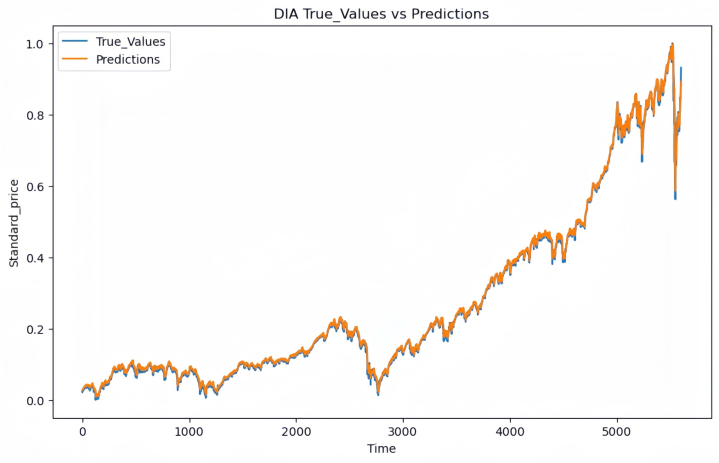
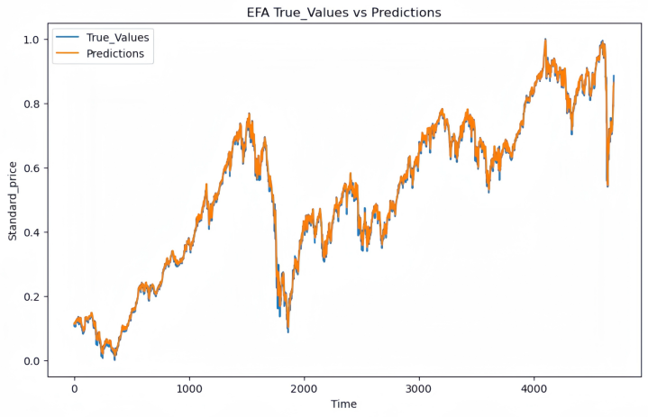
The typical MSE throughout these five stocks was 2.059e-04, recommending that the model generalizes well to hidden information with low prediction mistake. The relatively reduced MSE values in both training and test sets indicate the model's ability to catch patterns in everyday stock prices successfully.

4.2. High-Frequency Data Model

4.2.1. Model Design

For the high-frequency stock price prediction task, two LSTM versions were created to compare the influence of incorporating technical indicators. Both designs share the same design but differ in their input attributes. The initial version makes use of only minute-level stock price information, while the second version incorporates additional technical indicators to boost predictive efficiency.

No Technical Indicators Model: This version utilizes raw minute-level stock price information, consisting of open, high, reduced, close costs, and volume. The input series size is 5, implying the design uses data from the past five minutes to predict the next min's stock price. The LSTM layer has 12 concealed units, optimized with hyperparameter tuning to stabilize complexity and performance. A totally connected layer produces the last prediction.

With Technical Indicators Model: In addition to the 5 price attributes, this design integrates 6 technical indicators: Simple Moving Averages (SMA_3, SMA_5, SMA_10), Relative Strength Index (RSI), Moving Average Convergence Divergence (MACD), and the Signal Line. These indicators give more insights into market trends and energy, possibly improving the variation's capability to forecast short-term price activities. The input measurement increases from 5 to eleven with the incorporation of these indicators. The architecture remains similar to the initial design, utilizing an LSTM layer with 12 surprise devices followed by a completely connected layer. The specific same training method (50 dates, set dimension of 60, Adam optimizer) was used, guaranteeing a reasonable comparison in between the two models.

The addition of technical indicators boosts the input measurement from 5 to eleven, making it possible for the design to capture a more extensive understanding of market habits. By incorporating functions such as the Simple Moving Average (SMA), Relative Strength Index (RSI), and Moving Average Convergence Divergence (MACD), the design can represent both price energy and wider market trends, which could not be fully shown in price information alone. Both versions, with and without technical indicators, were trained and checked on the exact same dataset, with 80% of the information alloted for training and 20% for screening. This setup makes sure that any type of observed performance distinctions can be straight attributed to the presence or lack of technical indicators, utilizing a clear comparison of their result on prediction accuracy.

4.2.2. Experimental Results

The version integrating technical indicators achieved a typical accuracy of 39.79%, while the model without technical indicators achieved 39.12%. Although the increase in precision was moderate, the incorporation of technical indicators provided a small advantage in properly predicting stock price activities. On the other hand, the version without technical indicators performed much better in regards to evaluate loss. The normal test loss for the model without technical indicators was 0.01509, while the variation with technical indicators had a somewhat greater test loss of 0.02242. This recommends that, while the inclusion of technical indicators partially boosted accuracy, it also caused higher prediction mistake on the test collection.

Table 2: Model Performance Comparison

5. Conclusion and Future Work

In this study, I utilized Long Short-Term Memory (LSTM) networks to stock price prediction using both daily trading information and high-frequency minute-level information. The arise from the day-to-day trading information experiments demonstrated that the LSTM design carried out remarkably well, efficiently recording market trends. The dataset split in between training and testing sets showed to be trustworthy, enhancing the model's generalizability and making it better geared up to handle hidden information, which in turn increases its possible applicability to the more comprehensive stock market. The chosen training technique permitted the model to determine underlying market trends, giving beneficial insights for financiers.

For the high-frequency data, integrating technical indicators resulted in a slight enhancement in the version's ability to forecast stock price movements (i.e., whether the price would certainly climb, fall, or remain unchanged). However, this boost in classification precision was accompanied by a greater prediction mistake in regards to actual price values. The model that consisted of technical indicators showed a higher examination loss contrasted to the design relying solely on raw price information. This shows that while technical indicators may aid capture short-term trends, they can also introduce additional noise, leading to an overall increase in prediction error. This compromise highlights that the choice to incorporate technical indicators should depend on the details goals of the forecasting task. If the goal is to enhance classification accuracy for price activities, technical indicators supply a modest benefit. Nevertheless, if the focus gets on reducing price prediction errors, a version based solely on raw price data may confirm to be a lot more effective.

Looking ahead, this future research might check out using more diverse and detailed datasets to additionally improve version performance. Additionally, advanced strategies could be utilized for high-frequency information to reduce sound and improve both classification accuracy and price prediction accuracy. Crossbreed designs that integrate various other machine learning techniques with LSTM can additionally be investigated to attain a much better equilibrium between precision and loss.

References

[1]. Adya, A., Bahl, P., Padhye, J., Wolman, A., & Zhou, L. (2004). A Multi-Radio Unification Protocol for IEEE 802.11 Wireless Networks. Proceedings of the IEEE 1st International Conference on Broadband Networks (BroadNets'04), San Jose, CA, USA, 210–217. IEEE. https://doi.org/10.1109/BROADNETS.2004.8
[2]. Anzaroot, S., & McCallum, A. (2013). UMass Citation Field Extraction Dataset. Retrieved May 27, 2019, from http://www.iesl.cs.umass.edu/data/data-umasscitationfield
[3]. Fischler, M. A., & Bolles, R. C. (1981). Random Sample Consensus: A Paradigm for Model Fitting with Applications to Image Analysis and Automated Cartography. Communications of the ACM, 24(6), 381–395. https://doi.org/10.1145/358669.358692
[4]. Finn, C. (2018). Learning to Learn with Gradients. PhD Thesis, EECS Department, University of California, Berkeley.
[5]. Kleinberg, J. M. (1999). Authoritative Sources in a Hyperlinked Environment. Journal of the ACM, 46(5), 604–632. https://doi.org/10.1145/324133.324140
[6]. Van Gundy, M., Balzarotti, D., & Vigna, G. (2007). Catch Me, If You Can: Evading Network Signatures with Web-Based Polymorphic Worms. Proceedings of the First USENIX Workshop on Offensive Technologies (WOOT'07), Boston, MA, USA, Article 7, 9 pages. USENIX Association.
[7]. Demmel, J. W., Hida, Y., Kahan, W., Li, X. S., Mukherjee, S., & Riedy, J. (2005). Error Bounds from Extra Precise Iterative Refinement. Technical Report No. UCB/CSD-04-1344, University of California, Berkeley.
[8]. Harel, D. (1979). First-Order Dynamic Logic. Lecture Notes in Computer Science (Vol. 68). Springer-Verlag, New York, NY, USA. https://doi.org/10.1007/3-540-09237-4
[9]. Jerald, J. (2015). The VR Book: Human-Centered Design for Virtual Reality. Association for Computing Machinery and Morgan & Claypool.
[10]. Prokop, E. (2018). The Story Behind. Mango Publishing Group.
[11]. R Core Team. (2019). R: A Language and Environment for Statistical Computing. R Foundation for Statistical Computing. https://www.R-project.org/
[12]. Hochreiter, S., & Schmidhuber, J. (1997). Long Short-Term Memory. Neural Computation, 9(8), 1735–1780. https://doi.org/10.1162/neco.1997.9.8.1735
[13]. Fischer, T., & Krauss, C. (2018). Deep Learning with Long Short-Term Memory Networks for Financial Market Predictions. European Journal of Operational Research, 270(2), 654–669. https://doi.org/10.1016/j.ejor.2017.11.054
[14]. Chen, K., Zhou, Y., & Dai, F. (2015). A LSTM-Based Method for Stock Returns Prediction: A Case Study of China Stock Market. Proceedings of the IEEE International Conference on Big Data (Big Data 2015), Santa Clara, CA, USA, 2823–2824. IEEE. https://doi.org/10.1109/BigData.2015.7364089
Cite this article
Guo,H. (2024). Predicting High-Frequency Stock Market Trends with LSTM Networks and Technical Indicators. Advances in Economics, Management and Political Sciences,139,235-244.
Data availability
The datasets used and/or analyzed during the current study will be available from the authors upon reasonable request.
Disclaimer/Publisher's Note
The statements, opinions and data contained in all publications are solely those of the individual author(s) and contributor(s) and not of EWA Publishing and/or the editor(s). EWA Publishing and/or the editor(s) disclaim responsibility for any injury to people or property resulting from any ideas, methods, instructions or products referred to in the content.
About volume
Volume title: Proceedings of the 3rd International Conference on Financial Technology and Business Analysis
© 2024 by the author(s). Licensee EWA Publishing, Oxford, UK. This article is an open access article distributed under the terms and
conditions of the Creative Commons Attribution (CC BY) license. Authors who
publish this series agree to the following terms:
1. Authors retain copyright and grant the series right of first publication with the work simultaneously licensed under a Creative Commons
Attribution License that allows others to share the work with an acknowledgment of the work's authorship and initial publication in this
series.
2. Authors are able to enter into separate, additional contractual arrangements for the non-exclusive distribution of the series's published
version of the work (e.g., post it to an institutional repository or publish it in a book), with an acknowledgment of its initial
publication in this series.
3. Authors are permitted and encouraged to post their work online (e.g., in institutional repositories or on their website) prior to and
during the submission process, as it can lead to productive exchanges, as well as earlier and greater citation of published work (See
Open access policy for details).