1. Introduction

In the newly released Report on the Work of the Chinese Government, vigorously boosting consumption has been listed as the “top priority.” Promoting consumption is not only a core policy objective of the government but also a perennial theme in economics and management research. One of the key topics under this theme is identifying the factors that influence consumers' purchase decisions. Existing studies have proposed various consumer decision-making models, forming the theoretical foundation of consumer behavior. Among these, the POM model, proposed by Simonson and Rosen in 2014, identifies Personal Perception (P), Others' Evaluation (O), and Marketing (M) as the main factors influencing consumer purchasing behavior in the information age [1]. At present, few studies directly apply the POM model to investigate the determinants of consumer purchase decisions. However, findings in related literature can often be aligned with the POM framework. For example, Zou Bo et al. conducted a study on how consumers born in the 1980s choose smartphones. They found that factors such as the pursuit of trendiness, perceived price, group identity, and consumer innovativeness significantly influenced consumers’ decision-making processes. These influences can be categorized as P driven by O [2]. Similarly, Lai Hongbo, from a contextual perspective, examined how design-driven innovation in smart products affects perceived emotion and word-of-mouth communication. The results showed that aesthetic, semantic, and interactive dimensions of smart products all have significant positive effects on perceived emotion and word-of-mouth. Furthermore, elements of perceived emotion—such as pleasure and arousal (P)—play a mediating role between product design and word-of-mouth communication [3].

These findings suggest that the three factors in the model interact and combine in various ways to form different influence pathways. In other words, P, O, and M are not independent but rather interdependent and mutually influential, and there exist multiple paths that can lead to the same purchase decision outcome. Therefore, it is insufficient to simply propose influence pathways of type \( A_{3}^{3} \) composed of configurations of P, O, and M solely at the qualitative level. A more comprehensive approach combining qualitative and quantitative methods is needed to explore these interactions.

Qualitative Comparative Analysis (QCA) is a methodology that integrates qualitative and quantitative research to examine complex causal relationships and their configurations. QCA requires the analysis of factor combinations and adheres to several conditions: interdependence of factors, equivalence (multiple configurations leading to the same outcome), and asymmetry [4]. The interdependence and equivalence of factors are clearly present in consumer behavior, and while the presence of a particular factor may lead to a purchase decision, the absence of that factor does not necessarily mean a purchase will not occur—thus satisfying the condition of asymmetry. As such, QCA is suitable for studying the combined influence paths under the POM model. QCA is typically applied to small and medium-sized samples using survey data [5]. To enhance the method's relevance, this study focuses on a single product category: smartphones. Data collected through questionnaires are processed and then analyzed using fsQCA to perform calibration, necessity and sufficiency analysis, identifying core and peripheral conditions. After conducting robustness checks, the study derives multiple matching configurations for smartphone purchase decisions. However, QCA also has limitations. First, it is less suitable for large-sample analysis; when the number of conditions is low, an excessive number of cases may lead to the absence of logical remainders, causing complex, intermediate, and parsimonious solutions to converge. Second, the study scope is limited to smartphones. Third, QCA mainly serves as a bridge from qualitative to quantitative research and ultimately still requires precise quantitative analysis to measure the causal effects of different factors.

To extend the research to large samples and improve the scientific rigor of the results—while considering the challenge of observing P and the binary nature of the dependent variable—this study adopts the Generalized Structural Equation Model (GSEM). GSEM allows simultaneous prediction of P and regression analysis of consumer purchase behavior variables. Due to the difficulty in obtaining direct behavioral data on consumer purchases, implicit user feedback data from e-commerce platforms are used as a proxy. However, such datasets often lack proxy variables for O and M, as well as relevant control variables. In response, the study gathers two datasets and employs LightGBM and XGBoost methods to predict and impute missing values based on the variables shared between the datasets. Given the large sample size and model complexity, Python is used instead of Stata to efficiently generate the results.

2. Model construction

2.1. POM model

The POM model posits that consumer purchase decisions are shaped by the combined influence of three forces: Personal perception (P), Others’ evaluations (O), and Marketing efforts (M). Specifically, P refers to an individual's pre-existing preferences, beliefs, knowledge, and experiences; O encompasses the opinions of others and public information sources, including user reviews, advice from friends and family, media reports, expert opinions, and evaluations from third-party organizations; M denotes information provided by marketers, which includes advertisements, salespeople, distributors, packaging, branding, exhibitions, and other marketing channels [6]. Simonson and Rosen proposed a framework of combinational influence pathways to illustrate how these factors interact in consumer decision-making.

According to the existing framework, there are six identified patterns of combinational influence, classified based on the relative dominance of the three factors. The factor ranked first in each configuration is considered the dominant or driving force. Different configurations correspond to different industries or scenarios. For example, when a business places emphasis on marketing, a marketing-driven pattern emerges. This pattern is often seen in industries where consumers have a proactive demand for products or services, such as personal services or healthcare. In this context, marketing-driven influence gives rise to MPO and MOP configurations. The MPO pattern is suitable for scenarios with longer decision-making times. Consumers first learn about products through marketing, then compare options to enhance their personal cognition, and finally make a decision. In contrast, the MOP pattern suits scenarios with shorter decision-making times, where consumers make immediate purchase decisions after acquiring product information. Similarly, cognition-driven patterns lead to POM and PMO configurations, while word-of-mouth-driven patterns produce OPM and OMP configurations.

2.2. Qualitative Comparative Analysis (QCA)

This section introduces the method of Qualitative Comparative Analysis (QCA), outlining its advantages and applicability to this study, followed by a detailed account of the questionnaire design and data collection process. Questionnaire items were developed based on prior research and refined through a pilot study to ensure reliability and consistency. After revisions based on reliability and validity testing, the finalized questionnaire comprised nine measurement items and was distributed through online channels.

2.2.1. Overview and applicability of QCA

Qualitative Comparative Analysis (QCA), proposed by sociologist Ragin in 1987, is designed to explore causal relationships by examining the necessary and sufficient subset relationships between antecedent conditions and outcome variables [7,8]. QCA is well-suited for small samples (typically more than 30 cases) and is used to study complex causal relationships and their configurations. The method requires the analysis of configurations formed by multiple factors under the following conditions: interdependence, equivalence, and asymmetry. In the POM model, P, O, and M are interdependent and mutually influential, giving rise to multiple driving patterns in which any one factor may be a sufficient or necessary condition. Based on this analysis, QCA is deemed suitable for addressing the research questions in this study.

2.2.2. Questionnaire and variable design

This study selects personal preference, others’ evaluation, and marketing strategies as antecedent conditions, aiming to explore how combinations of these factors jointly influence consumers' purchase decisions. First, the questionnaire items were developed with reference to validated scales in domestic and international studies and tailored to the POM framework. Next, the initial items were revised based on expert feedback and small-scale interviews with the target population. Finally, a pilot test was conducted to assess the reliability and validity of the questionnaire, leading to the finalized version.

The questionnaire is composed of three parts with a total of eight items: Part I provides background information and introduces the concepts of the POM model; Part II gathers demographic information such as gender, age, education level, and income; Part III, the core section, begins with a screening question to determine whether the respondent is considering purchasing a smartphone, establishing the basis for the outcome variable. This is followed by questions measuring the influence of P, O, and M using a five-point Likert scale (ranging from “strongly disagree” to “strongly agree”).

The outcome variable is clearly defined: whether the consumer ultimately decides to purchase a smartphone under the combined influence of P, O, and M. Responses of “yes” are coded as 0, and “no” as 1, then calibrated into a crisp set for QCA.

For the condition variables: P (Personal perception) includes three items: ac, ba, cc, corresponding to Question 6 (e.g., “To what extent is your choice influenced by your own subjective preferences?”); O (Others' evaluations) includes three items: dc, ec, fc, corresponding to Question 7; M (Marketing) includes three items: gc, hc, ic, corresponding to Question 8. All condition variables are measured on a five-point Likert scale and treated as fuzzy sets. Therefore, they cannot be directly assigned binary values of 0 or 1, but must be calibrated into values between 0 and 1.

The mapping between condition variables and questionnaire items is illustrated in the figure below:

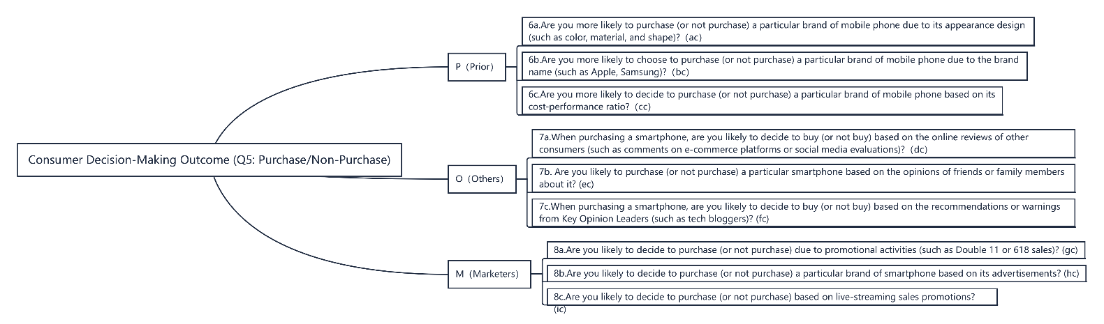
Figure 1: QCA variable selection diagram

2.3. Generalized Structural Equation Model (GSEM)

The QCA approach adopts a relatively subjective perspective by analyzing small-sample survey data on smartphone purchases to identify the configurational paths of the POM model and derive suitable consumer decision-making configurations. Naturally, it is necessary to examine whether these configurations can be generalized to large samples and to apply more quantitative methods to analyze the effects of different configurations. Therefore, regression analysis can be conducted on the POM model and its configurations. In the regression model, the core explanatory variables are \( P,O,M \) ,while the binary dependent variable \( Y \) denotes consumer behavior, where \( Y=0 \) indicates no purchase and \( Y=1 \) indicates a purchase. \( r \) control variables \( W \) are introduced to construct a preliminary binary Logit regression model as follows:

\( Logit({Y_{i}})={β_{0}}+{β_{1}}{P_{i}}+{β_{2}}{O_{i}}+{β_{3}}{M_{i}}+{β_{4}}{W_{1i}}+...+{β_{3+r}}{W_{ri}}+{u_{i}} \) (1)

Among the explanatory variables, \( O \) and \( M \) can be represented using corresponding proxy variables. However, \( P \) —representing personal perceptions and beliefs—is a latent and difficult-to-observe variable. Generally, researchers may adopt panel data with fixed effects regression to control for omitted variable bias. However, when the unobserved variable is not an omitted variable but a key explanatory variable itself, fixed effects models are ineffective, as the causal effect \( {β_{1}} \) cannot be directly estimated. Similarly, using instrumental variables for two-stage regression is impractical in this case, as the first-stage regression still requires data for \( P \) . Thus, we consider applying the Structural Equation Model (SEM), treating \( P \) as a latent variable and estimating its value using observable variables \( X \) that are associated with personal perception. The simplified structural equation model is therefore constructed as follows:

\( \begin{cases} \begin{array}{c} {P_{i}}={λ_{1}}{X_{1i}}+{λ_{2}}{X_{2i}}+...+{λ_{k}}{X_{ki}}+{ε_{i}} \\ {Y_{i}}={β_{0}}+{β_{1}}{P_{i}}+{β_{2}}{O_{i}}+{β_{3}}{M_{i}}+{β_{4}}{W_{1i}}+...+{β_{3+r}}{W_{ri}}+{u_{i}} \end{array} \end{cases} \) (2)

In this model, Equation (1) is the measurement model, where \( X \) represents observable variables associated with personal perception \( P \) , and Equation (2) is the structural model. Regression on this simplified model reveals that the coefficients are not statistically significant. The significance of the model is affected by the functional form of the equations and the selection of variables \( X \) and \( W \) . First, since \( Y \) is a binary dependent variable, the linear probability model must be replaced with a Logit model. It is important to note that standard SEM models are only suitable for continuous dependent variables, and therefore need to be adjusted to a Generalized Structural Equation Model (GSEM) to accommodate binary dependent variables with appropriate distribution and link functions. Second, the functional form of the model can be improved based on economic rationale. The lack of significant coefficients may be due to the model overlooking nonlinear relationships or interaction effects between variables. To address this, a nonlinear term \( {P^{2}} \) can be introduced. The influence of personal perception \( P \) on purchase decisions may not be linear; for example, both very low and very high perceptions might lead to non-purchase, with the highest purchase intention occurring at moderate levels of perception. This type of nonlinear effect is common in consumer behavior research. In addition, interaction terms such as \( P×O \) can be included. Personal perception \( P \) and others’ evaluations \( O \) may exhibit complementary or substitutive effects. For instance, consumers with high perceptions may rely more on their own judgment, while those with low perceptions may be more influenced by external evaluations. In terms of variable selection, the empirical analysis collected multiple candidate variables. Based on economic meaning, the following variables are preliminarily selected:

Table 1: Variable selection table

The selected \( X \) variables encompass three dimensions—behavior (time, page views), preference (category preference, interests), and consumption (average price, total spending)—to comprehensively reflect the formation process of P, thus avoiding the limitations of a single dimension. The \( W \) variables cover basic consumer characteristics and environmental factors [10], clearly distinguished from \( P,O,M \) to prevent multicollinearity or endogeneity. Other variables and data were also collected during the data collection process, but were excluded for various reasons. For instance, cate (purchased product category) and brand (product brand) are more likely to be outcomes of purchase decisions \( Y \) rather than indicators of \( P \) , and thus were excluded to avoid reverse causality. Comment_num (number of product reviews) and has_bad_comment:(presence of negative reviews) are related to others' evaluations ( \( O \) ) and should not be included in the measurement of \( P \) .Last_Login_Days_Ago (days since last login) mainly reflects user activity and is weakly related to perception.

Finally, to better utilize the results of the QCA configurations and achieve methodological integration, it is necessary to map the QCA conditions to the GSEM model variables. The QCA conditions (cc, dc, ic) must be aligned with the GSEM variables (P, O, M). Based on variable definitions and semantics, we can make the following assumptions: product performance (cc) corresponds to P (personal perception), which is constructed from TSSM, PV, PCP, etc., reflecting consumers’ perceptions of product function and value and is closely related to cc; brand evaluation (dc) corresponds to O (others’ evaluations), representing social influences (such as peer recommendations, social media reviews), consistent with dc; price (ic) corresponds to M (enterprise marketing), including pricing strategies, promotions, and other marketing tactics relevant to ic.

Next, interaction terms should be assigned according to configurational characteristics, mapping QCA configuration traits to model parameters. The interaction term \( P×O \) , already included in the model, captures the synergy between personal perception and brand evaluation. Additionally, new interaction terms such as \( P×M \) (representing the interaction between personal perception and enterprise marketing) and \( O×M \) (representing the joint effect of brand evaluation and marketing efforts) need to be added.

Ultimately, we obtain an improved GSEM model incorporating real variables.

\( \begin{cases} \begin{array}{c} {P_{i}}={λ_{1}}TSS{M_{i}}+{λ_{2}}P{V_{i}}+{λ_{3}}PC{P_{i}}+{λ_{4}}Interest{s_{i}}+{λ_{5}}AO{V_{i}}+{λ_{6}}T{S_{i}}+{ε_{i}} \\ Logit({Y_{i}})={β_{0}}+{β_{1}}{P_{i}}+{β_{2}}{O_{i}}+{β_{3}}{M_{i}}+{β_{4}}{{P_{i}}^{2}}+{β_{5}}({P_{i}}×{O_{i}})+{β_{6}}({P_{i}}×{M_{i}})+{β_{7}}({O_{i}}×{M_{i}}) \\ +{β_{8}}ag{e_{i}}+{β_{9}}se{x_{i}}+{β_{10}}Incom{e_{i}}+{β_{11}}Locatio{n_{i}}+{β_{12}}lv\_c{d_{i}}+{u_{i}} \end{array} \end{cases} \) (3)

3. Data processing and configurational analysis

3.1. Descriptive statistics and questionnaire quality assessment

First, SPSS 23.0 was used to analyze the characteristics of the 100 valid responses collected through the formal questionnaire. According to the analysis results, more than half of the respondents in the smartphone purchase decision sample were aged between 19 and 30, which aligns with the actual age structure of the main smartphone consumer group. In terms of educational background, the majority of respondents had a college degree or below, accounting for 84%, with the rest evenly distributed across other education levels. The distribution of average monthly disposable income was relatively balanced, indicating that the sample represented a wide range of consumer spending levels. Regarding the premise of the survey—"choosing whether or not to purchase a smartphone"—the ratio of purchase to non-purchase was close to 1:1, suggesting a balanced distribution of the outcome variable.

Reliability and validity tests were conducted on the questionnaire. Reliability assesses the stability of the measurement scale—higher reliability indicates greater stability [11]. Internal consistency reliability was examined for the scales used in the study, and the results are shown in Table 2. The reliability of each variable’s scale, as well as the overall reliability, exceeded 0.6. The Corrected Item-Total Correlation (CITC) values were generally above 0.5, and deleting any item did not lead to a significant increase in Cronbach’s alpha, indicating that all items should be retained [12]. These findings suggest that the formal questionnaire demonstrates good consistency and stability, and all measurement items are suitable for subsequent analysis.

Table 2: Reliability test

Validity was tested using the Kaiser-Meyer-Olkin (KMO) measure and Bartlett’s test of sphericity. The results, presented in Table 3, show that the KMO values for all three latent variables exceeded 0.6. Bartlett’s test reached significance at the 0.05 level [13], and the overall KMO value was 0.840. The results of Bartlett’s test were also statistically significant, indicating that the questionnaire data were suitable for factor analysis.

Table 3: Validity test

3.2. Data calibration

Calibration is the process of assigning set membership scores to cases, aiming to determine the degree to which each case belongs to a fuzzy set. For data collected through questionnaire surveys, calibration is typically carried out by setting thresholds for full membership, full non-membership, and a crossover point. Cases with a membership score of 1 are fully in the set, while those with a score of 0 are fully out of the set, and the crossover point marks the boundary between the two [14].

For the 5-point Likert scale used in this study, some researchers directly adopt the maximum point (5), midpoint (3), and minimum point (1) as the three qualitative anchors [15]. While this method reflects the inherent meaning of the questionnaire items to some extent, it may not suit the distributional characteristics of the current dataset. Using the 95th and 75th percentiles for calibration, for instance, leads to identical membership and crossover points, resulting in too many cases calibrated at 0.5. To address this issue, this study draws on the calibration approach proposed by Ilias O. Pappas and Arch G. Woodside [16], setting the values 4, 3, and 2 as the three qualitative anchors, and assigning a membership score of 0.95 to the value 4. This method better reflects actual response patterns in the questionnaire data. Based on the established anchors, the data were imported into fsQCA 3.0 software, and the values of each variable were converted into set membership scores ranging from 0 to 1.

3.3. Configurational analysis

3.3.1. Necessity analysis

Before conducting the analysis of condition configurations, it is necessary to examine the necessity of each individual condition. In line with mainstream QCA studies, this study first tests whether any single condition constitutes a necessary condition for consumers’ decisions to purchase smartphones. Necessity analysis examines the extent to which the outcome set is a subset of the condition set—i.e., whether the occurrence of the outcome Y always requires the presence of condition X. In QCA, if a condition is always present when the outcome occurs, it is considered a necessary condition for that outcome.

After calibration, necessity analysis of the outcome was performed using fsQCA. The outcome variables were denoted as y and ~y (i.e., the negation of y). The consistency of each antecedent condition was used as the evaluation criterion. A consistency score greater than 0.9 indicates that the condition may be necessary for the occurrence of the outcome Y. In this context, consistency refers to the degree to which the condition is necessary for the outcome, while coverage indicates the empirical relevance of the condition. The consistency is calculated as \( Consistency({X_{i}}≤{Y_{i}})=\sum [min{(}{X_{i}},{Y_{i}})]/\sum ({X_{i}}) \) , and the coverage as \( Coverage({Y_{i}}≤{X_{i}})=\sum [min{(}{X_{i}},{Y_{i}})]/\sum ({Y_{i}}) \) ,where \( {X_{i}} \) represents the calibrated value of the condition and \( {Y_{i}} \) represents the calibrated value of the outcome.

Given the threshold of 0.9 for consistency, a condition is deemed necessary only if its consistency exceeds this threshold. Based on the analysis results, all conditions had consistency levels below 0.9. Therefore, no single condition can be identified as a necessary condition for influencing consumers’ decisions to purchase a particular smartphone.

3.3.2. Sufficiency analysis

To explore how antecedent conditions interact to influence smartphone purchase decisions, this study employed the fsQCA 3.0 software to conduct a sufficiency analysis. The aim was to identify multi-condition configurations (i.e., pathways) that lead to the outcome and to perform both vertical (within-path) and horizontal (cross-path) comparisons to uncover the complex causal mechanisms involved.

The first step involved setting thresholds for case frequency and consistency. The case frequency threshold refers to the minimum number of cases required for a configuration to be considered in the analysis. When the sample size is relatively large, this threshold should be raised to exclude outlier cases, but at least 75% of the original cases should be retained. Some scholars recommend that the case frequency threshold be approximately 1.5% of the total sample size [17]. Given that this study collected 100 valid cases, the case frequency threshold was set to 1, thereby retaining more than 75% of the sample. The raw consistency threshold reflects the minimum acceptable level of association between a configuration of antecedent conditions and the outcome. Configurations with raw consistency scores greater than or equal to the threshold are considered subsets of the outcome set and assigned a value of 1; otherwise, they are assigned 0. Most existing studies suggest setting the raw consistency threshold at 0.8. Another filtering criterion is PRI consistency, which evaluates the extent to which the data exhibit causal asymmetry (i.e., different causes leading to the same result). The commonly accepted threshold for PRI consistency is 0.7 [18]. Therefore, this study set the raw consistency threshold at 0.8 and the PRI consistency threshold at 0.7 and conducted configurational analysis using fsQCA 3.0.

The fsQCA output includes three types of solutions: complex, intermediate, and parsimonious. Among these, the intermediate solution strikes a balance between empirical relevance and theoretical plausibility—it simplifies the results without contradicting real-world conditions. Thus, intermediate solutions are commonly used to identify the condition configurations that lead to the outcome. The parsimonious solution helps differentiate between core and peripheral conditions. In this study, the intermediate and complex solutions yielded the same results for smartphone purchase decisions, indicating a high level of logical consistency in the model. Details are shown in Table 4.

Table 4: Intermediate and complex solutions for purchasing decisions

According to the configurational result expression method proposed by Ragin, if a condition appears in both the intermediate and parsimonious solutions, it is regarded as a core condition, indicating a strong causal relationship between the condition and the outcome. If a condition appears only in the intermediate solution, it is identified as a peripheral condition, suggesting a weaker causal link. Given that the intermediate and complex solutions in this study are consistent, the classification of core and peripheral conditions is based on the frequency of their appearance in the configurations and their relative strength of influence on the outcome. In Table 5, the following symbols are used to represent the presence or absence of conditions: ●: presence of a core condition; •: presence of a peripheral condition; ⊗: absence of a core condition; ○: absence of a peripheral condition; Blank: the presence or absence of the condition is not relevant.

Since condition “cc” appears positively in all three configurations with the highest frequency and consistent form, it is identified as a core condition. Conditions “dc” and “ic” demonstrate high consistency when present but appear in both affirmative and negated forms across configurations, so they are classified as peripheral conditions. The overall consistency of the three configurations is 0.910912, which exceeds the required threshold of 0.8. Robustness tests were also conducted by increasing the consistency threshold, PRI threshold, and frequency threshold. Ultimately, three viable configurational paths for smartphone purchasing decisions were identified, as shown in Table 5.

Table 5: Configurations of purchase decisions

Note: ● = core condition present; ⊗ = core condition absent; • = peripheral condition present;  = peripheral condition absent.

Configuration 1: Rational Decision-Maker: ~ac*~bc*cc*~dc*~ec*~fc*~gc*~hc*~ic, In this configuration, “cc” (product performance) is the core condition, while the absence of peripheral conditions “dc” (brand evaluation) and “ic” (price) indicates that consumers are relatively insensitive to these aspects. This type of consumer—rational decision-makers—primarily bases their decision on product functionality rather than additional brand or pricing factors.

Manufacturers should emphasize core technical features such as processor speed and battery life. These consumers respond well to objective, data-driven product specifications and expert reviews, and are less influenced by promotional pricing or brand imagery.

Configuration 2: Brand-Oriented Type: ~ac*bc*cc*dc*~ec*fc*~gc*~hc*ic. In this configuration, “cc” remains the core condition, with “dc” and “ic” present as peripheral conditions. These consumers can be characterized as brand-loyal; they prefer familiar or trusted brands and value both product performance and supplementary services such as after-sales support. They are also more likely to be influenced by peer recommendations or social media evaluations.

Manufacturers should invest in brand building and loyalty programs. High-quality customer service (e.g., warranty extensions, repair guarantees) can help attract and retain this consumer group. Social media marketing and endorsements from key opinion leaders (KOLs) or influencers are also effective.

Configuration 3: Comprehensive Evaluator: ac*bc*cc*dc*ec*fc*gc*hc*~ic. In this configuration, “cc” is the core condition, with “dc” as a peripheral condition and “ic” (price) absent. These consumers—comprehensive evaluators—take into account a wide range of factors, including performance, brand, design, promotion, and after-sales service. They are less dependent on external opinions and base their decisions on a holistic personal evaluation.

Firms should offer high-value products that balance price and performance. Marketing strategies should highlight multiple dimensions of the product—such as brand strength, aesthetics, promotional offers, and customer support. Rather than relying heavily on external endorsements, the product’s integrated quality and value proposition will drive consumer preference.

4. Empirical analysis

The empirical analysis for the GSEM model is conducted using two datasets: the JD.com algorithm competition dataset and the Whale Community e-commerce user behavior dataset. These datasets contain various data, including user behavior, product review rates, subscription status to enterprise advertisements, as well as demographic variables such as gender and age, which are highly relevant to the research model. The JD.com dataset comprises 105,321 records of user information, 24,187 product records, 558,552 review records, and 13,199,934 user behavior records. The e-commerce user behavior dataset consists of 1,000 records of user demographic and behavioral data.

4.1. Data preprocessing

Each dataset was processed separately. For the JD.com dataset, Excel Power Query was employed for conditional data merging, linking user, product, and review data using the common identifiers user_id and sku_id. The resulting data was then filtered based on specific columns. The type column, which represents user behavior, was categorized into six types: 1 for browsing, 2 for adding to the shopping cart, 3 for removing from the cart, 4 for completing a purchase, 5 for adding to favorites, and 6 for clicking. After statistical analysis, it was found that the majority of observations related to behavior type 6 are only indicative of browsing, which typically precedes other actions. Therefore, data were filtered to retain only behavior types 1 and 4, with type 1 representing non-purchase behavior (buy=0) and type 4 representing purchase behavior (buy=1). Further, redundant data were present due to discrepancies in the "dt" column (representing comment dates). Given that most purchases were made around April 1 and 2, 2016, data prior to March 28, 2016, was selected to ensure completeness of product reviews visible to users at the time of their purchase decisions. After filtering, duplicate entries remained where users had purchased multiple items, which was deemed valid. The data were then sorted by user_id, resulting in a final dataset containing 101,706 entries. To facilitate regression analysis in Stata, additional transformations were applied: missing values marked as "-1" were handled, the sex column values of "2" were treated as missing, and the type column was renamed as buy, with the conversion type=1 to buy=0 (non-purchase) and type=4 to buy=1 (purchase). Furthermore, the age column was transformed into a categorical variable, spanning five categories. The relevant variables available for analysis included: buy as the dependent variable, bad_comment_rate (product review rate) as the independent variable O, with other variables serving as potential control variables.

For the e-commerce user behavior dataset, data transformations were primarily focused on the creation of the Interest, Product_Category_Preference, and Newsletter_Subscription columns (with the latter renamed as M, corresponding to the independent variable M). Additional transformations were applied to age and sex to create categorical variables for regression analysis. Despite both datasets sharing the same user_id, they originated from different sources, and merging them directly resulted in a dataset with many missing values. Specifically, the JD.com dataset lacked certain columns from the e-commerce dataset, such as Location, Income, Interest, Average_Order_Value, Total_Spending, Product_Category_Preference, Time_Spent_on_Site_Minutes, Pages_Viewed, and M. These missing columns were not crucial for the study, and imputation was focused on the relevant missing values.

4.2. Handling missing data

After observing the missing columns, it was found that the Location column, which represents geographic regions, is relatively independent of other columns, whether known or unknown. Directly adding it to the primary prediction model may negatively affect the overall prediction accuracy. Furthermore, M, as the explanatory variable in the regression model, is the most critical and closely monitored column for imputation. Therefore, the imputation process should prioritize the most accurate prediction of M. Consequently, the imputation order was designed as follows: first, impute the Location column, followed by other columns, and finally impute M. The Location column contains only the values 1, 2, and 3. To impute missing values, the known data distribution was first calculated to create a probability distribution, and then missing values were randomly filled based on this distribution.

Next, LightGBM was used to perform multiple imputation for the remaining missing columns. Missing values are a common issue in data analysis and machine learning tasks, directly impacting model performance and predictive accuracy. In this task, the missing data consists of mixed types, including both categorical and numerical variables, and the dataset is large, containing more than 100,000 rows. There are potential relationships between data columns, such as between Income and Total_Spending. The known columns in this task are age, sex, and Location. Traditional imputation methods (such as mean imputation, mode imputation, or KNN-based imputation) are too simplistic and do not fully exploit the relationships between data. Given the characteristics of the data, this study introduces an imputation method based on LightGBM, which uses machine learning models to predict missing values based on known features, improving both data completeness and prediction accuracy. LightGBM natively supports categorical variables (no need for manual encoding), efficiently handles mixed-type data, and is robust to missing values. It is particularly suited for large-scale datasets, outperforming random forests in terms of training speed and memory usage. In terms of accuracy, LightGBM typically achieves comparable precision to XGBoost, but with faster speed.

LightGBM uses the LGBMClassifier to handle categorical features and the LGBMRegressor to process numerical features. By identifying and marking both known and unknown data, the model is trained using the known features to predict the missing values in the target column. The imputation is performed iteratively, filling the missing columns one by one in a predefined order, and each filled column is then treated as a new feature for predicting subsequent columns. The detailed implementation steps are as follows: 1. Basic Feature Preprocessing: Missing values in the known columns (age, sex, and Location) are marked as -1 and converted into categorical types. 2. Defining Target Columns and Imputation Order: The target columns are defined (as either categorical or numerical variables), and the imputation order is specified, prioritizing the use of basic information (such as interest and preference) to fill other related columns. 3. Core Function for Missing Value Imputation: This step involves several processes: Data Identification: Extract the known data and mark the rows that need to be filled; Handling Extreme Cases: If there is no known data, the categorical column is filled with the global mode, and the numerical column is filled with the global mean. If fewer than 50 known data points exist, the categorical column is filled with the local mode and the numerical column with the local mean. This degrades to statistical imputation to enhance the model’s robustness; Data Preparation: Extract the feature matrix and target vector. If the dataset contains more than 100 rows, 20% of the data is set aside as a validation set; otherwise, the full dataset is used for training; Model Configuration: Includes setting up the classifier, regressor, and optimizing parameters; Model Training: Early stopping is used to prevent overfitting, with the stopping rounds set to 50 [19]. Categorical features are specified to improve performance; Prediction and Imputation: Missing rows are predicted, and Gaussian noise (with a standard deviation of 0.5 times the standard deviation of the target column) is added to numerical predictions to avoid deterministic filling, with the predictions truncated to a reasonable range. 4. Feature Engineering and Iterative Imputation: Features like sex, age, and Location are used, and interaction terms like loc_sex are created to capture potential relationships. The imputation proceeds iteratively according to the fill_order. After each filling step, the target column is added to the current features for subsequent predictions, ensuring that loc_sex is not added more than once. 5. Cleanup and Saving: After the imputation process, auxiliary columns are deleted, and the new data file is saved.

Finally, the XGBoost model was used to impute the missing values in column M, which is a binary variable with values of 0 or 1. The objective of this task was to predict and fill in the missing M values by leveraging the relationships among existing features in the dataset. XGBoost, a machine learning algorithm based on gradient-boosted decision trees, offers high predictive performance, suitability for classification tasks, robustness, efficiency, and flexibility [20]. Specifically, XGBoost integrates multiple decision trees to capture non-linear relationships and complex patterns among features. It optimizes predictive accuracy through log-loss and is more appropriate than traditional statistical approaches (e.g., mean imputation) for predicting the categorical variable M. Moreover, XGBoost demonstrates strong robustness against noise and outliers, supports parallel computation, and is well-suited to large-scale datasets that may contain imperfect data. Lastly, XGBoost offers a wide range of hyperparameter tuning options (e.g., learning rate, tree depth), allowing performance optimization based on specific task requirements. Compared with linear regression or simple interpolation methods, XGBoost has significant advantages in capturing multivariate relationships and handling categorical targets, making it the optimal choice for this task. The method can be summarized into five steps: data preprocessing, dataset splitting, model training, and missing value prediction. 1. Data Loading and Preprocessing: Missing values were replaced and treated as a separate category. Features were divided into categorical and numerical types. 2. Dataset Splitting: Training and Prediction Sets: It was assumed that the last 1,000 rows contained complete values of M and were used as the training set; the first 101,706 rows with missing M values were used as the prediction set. Features and Target: Feature matrix X_train and target variable y_train were extracted from the training set, while the prediction feature matrix X_predict was obtained from the prediction set. 3. Feature Preprocessing: A ColumnTransformer was used to apply one-hot encoding to categorical features, while numerical features remained unchanged. The parameter handle_unknown='ignore' was set to avoid errors during prediction when encountering unseen categories. 4. Model Pipeline Construction: A Pipeline was built to integrate preprocessing with the XGBoost classifier, streamlining the process and ensuring consistency. The model was configured with eval_metric='logloss' to use log-loss as the evaluation metric for classification. 5. Model Training and Prediction: The model was trained using X_train and y_train. Predictions were made on X_predict, resulting in y_pred, i.e., the imputed values for M. Finally, the predicted results were filled back into the original dataset for the first 101,706 rows.

4.3. GSEM model regression results

After importing the processed data into Stata and running the GSEM model, it was found that due to the large dataset and the involvement of binary Logit regression, the software calculations were slow and could not iterate to the optimal result. Therefore, the model was implemented in Python using PyCharm. Before obtaining the results, it was necessary to clarify the regression outcomes corresponding to different configuration types for each coefficient:

Table 6: Configuration results adapted to the GSEM model

The results from the regression model were exported into a Word document, which includes the above configuration table.

Table 7: Regression results of the measurement model

Variables like Location:2 and PCP_2 are dummy variables generated after applying one-hot encoding using pd.get_dummies function and statsmodels. Dummy variables are a way to convert categorical variables into numerical forms. Since categorical variables cannot be directly fed into mathematical models, a set of binary variables (0 or 1) is created to represent each category.

Regression Results: The regression results show that the time users spend on the platform, the number of pages they browse, the average order price, and the total expenditure significantly impact users' personal perceptions. Considering the coefficients, it can be seen that the longer users spend on the platform and the more pages they browse, the more likely their perceptions and beliefs will be influenced. However, the total and average expenditure on the platform has relatively less impact.

Furthermore, according to the results of the structural model, personal perception \( P \) is precisely a significant influencing factor in users' purchase decisions and exhibits a clear nonlinear pattern. Other variables are not statistically significant, indicating that \( O \) (negative review rate) and \( M \) (whether the user subscribes to enterprise marketing campaigns) do not play a decisive role in the purchasing decision. In addition, the interaction effects among \( P,O,M \) are also not significant, suggesting that \( P \) is not sensitive to either \( O \) or \( M \) .These findings indicate that, in a large sample without restrictions on the product being purchased, the rational decision-making type represents the more dominant consumer group.

5. Conclusion and recommendations

This study, based on the POM theoretical framework, combined with QCA and GSEM methods, systematically explores the influencing mechanisms of consumer purchase decisions in dynamic market environments. Through empirical analysis of the JD.com algorithm competition dataset and e-commerce user behavior data, the following key conclusions were drawn:

(1) Core Driving Role of Personal Perception (P): Consumer personal perception (including time spent on the platform and page views) has a significant positive impact on purchase decisions and shows non-linear characteristics. The information acquisition and processing behaviors of consumers on the platform (such as time investment and information breadth) directly shape their product cognition, thereby leading and influencing the rational decision-making process. This conclusion validates the dominant role of personal factors in the POM model in an environment with information transparency.

(2) Limited Impact of Others' Evaluation (O) and Corporate Marketing (M): The direct effects of the review rate and subscription to marketing information, as well as their interaction effects, were not significant. This indicates that in a large sample generalization scenario, consumers have low sensitivity to social evaluations and marketing information. This could be due to the proxy variables for O and M in the data not fully capturing the actual influence dimensions, or consumers may have developed a rational filtering mechanism for marketing information after years of shopping experience.

(3) Dominance of Rational Decision-Making Model: The GSEM regression results indicate that consumers are more likely to rely on their personal experience and information processing abilities to make decisions rather than being driven by external evaluations or short-term marketing strategies. This finding is consistent with the "rational decision-making" configuration identified in the QCA small sample analysis, confirming the universality of the research hypothesis in large samples.

Based on the above conclusions, the following management recommendations and research directions are proposed:

(1) Focus on Core Product Development: Enterprises should attract consumers by improving the core performance of products (such as technology and appearance) and continually optimize their products based on consumer preferences.

(2) Optimize Consumer Information Reach: Enterprises should enhance product information transparency and user experience (e.g., optimizing page design, increasing user stay time, and enhancing personalized recommendations) to deepen consumers' personal perceptions. For example, behavioral data analysis can be used to understand user interests and dynamically adjust information display strategies to reinforce positive perception accumulation.

(3) Refined Marketing Strategy Design: Although the direct effect of corporate marketing (M) is limited, its potential synergistic effect with personal perception deserves attention. It is recommended to develop differentiated marketing combinations (e.g., targeted pricing strategies, contextual advertising) based on user profiles and explore the dynamic interaction mechanism between P and M to avoid resource wastage from a one-size-fits-all marketing approach.

(4) Improvement of Data Collection and Variable Measurement: Future research should improve the design of proxy variables for others' evaluations (O) and corporate marketing (M), for instance, by incorporating social media sentiment analysis, marketing content sentiment analysis, etc., to capture the multidimensional effects of external factors more accurately. Additionally, research can be extended to other industries (such as fast-moving consumer goods and durable goods) to validate the robustness of the conclusions across different scenarios.

(5) Methodological Integration and Theoretical Expansion: Further integration of QCA's configurational thinking and GSEM's quantitative analysis advantages is needed to explore the complex paths of multi-factor non-linear relationships. Moreover, introducing moderating variables like cultural background and product type can deepen the understanding of boundary conditions in the POM model, providing a more dynamic and adaptable analytical framework for consumer behavior theory.

Acknowledgment

Chaojie Fan and Meng Gu: Conceptualization, Methodology, Data curation, Writing- Original draft preparation, Visualization, Investigation.

References

[1]. Author(s): N/A. (2014). Absolute value: What really influences customers in the age of (nearly) perfect information (Hardcover). Bargain Price.
[2]. Zou, B., & Lee, K.-H. (2011). An empirical study on the factors influencing the purchase intention of innovative products among post-80s consumers: A case study of smartphones. China Market, (26), 9-10+29.
[3]. Lai, H.-B., & Yang, Z.-C. (2023). The impact of design-driven smart product innovation on perceived emotions and word-of-mouth communication from a scenario perspective. Science and Technology Progress and Countermeasures, 40(24), 31-40.
[4]. Ni, T.-C., Zhu, R.-P., Huang, Y., et al. (2022). The differences in media trust attribution under Hofstede's cultural dimensions: A study based on data from 24 European countries. International Journalism, 44(06), 27-49. https://doi.org/10.13495/j.cnki.cjjc.2022.06.005
[5]. He, J.-W., Liu, X.-T., Zhou, Z.-H., et al. (2024). A study on the driving mechanism of kindergarten teachers' vision development: Based on fuzzy-set qualitative comparative analysis. Early Childhood Education Research, (02), 42-53. https://doi.org/10.13861/j.cnki.sece.2024.02.006
[6]. Zhou, B. (2019). Application of POM theory in marketing practice. China Market, (25), 4-6+8.
[7]. Ragin, C. C., & Fiss, P. C. (2008). Net effects analysis versus configurational analysis: An empirical demonstration. In Redesigning Social Inquiry: Fuzzy Sets And Beyond (pp. 190-212).
[8]. Fiss, P. C. (2011). Building better causal theories: A fuzzy set approach to typologies in organization research. Academy of Management Journal, 54(2), 93-420.
[9]. Yu, X., Li, B.-L., & Qiao, J. (2013). Analysis of factors influencing consumers' cognition, purchasing behavior, and purchasing intention toward mid- to high-end pork: A survey of urban residents in Beijing. China Animal Husbandry Journal, 49(12), 24-29.
[10]. Chen, B.-J., Guo, K.-M., Chen, F.-F., et al. (2023). Remaining useful life prediction of aircraft engines based on residual NLSTM network and attention mechanism. Journal of Aerospace Power, 38(05), 1176-1184. https://doi.org/10.13224/j.cnki.jasp.20210728
[11]. Wu, M.-L. (2010). Questionnaire statistical analysis practice: SPSS operation and application. Chongqing: Chongqing University Press.
[12]. Zhou, J., & Ma, S.-P. (2024). SPSSAU research data analysis methods and applications (1st ed.). Electronic Industry Press.
[13]. Chung, R. H., Kim, B. S., & Abreu, J. M. (2004). Asian American multidimensional acculturation scale: Development, factor analysis, reliability, and validity. Cultural Diversity and Ethnic Minority Psychology, 10(1), 66-80.
[14]. Ragin, C. C. (2009). Redesigning social inquiry: Fuzzy sets and beyond. University of Chicago Press.
[15]. Fiss, P. C. (2011). Building better causal theories: A fuzzy set approach to typologies in organization research. Academy of Management Journal, 54(2), 393-420.
[16]. Pappas, I. O., & Woodside, A. G. (2021). Fuzzy-set qualitative comparative analysis (fsQCA): Guidelines for research practice in Information Systems and marketing. International Journal of Information Management, 58, 102310.
[17]. Rihoux, B., & Ragin, C. C. (2008). Configurational comparative methods: Qualitative comparative analysis (QCA) and related techniques. Sage Publications.
[18]. Zhang, M., & Du, Y.-Z. (2019). Application of QCA method in organizational and management research: Positioning, strategy, and direction. Journal of Management Studies, 16(9), 1312-1323.
[19]. Wang, H.-W., & Xia, Y.-Q. (2009). An empirical study on the factors influencing customer trust in online shopping. Journal of Intelligence, 28(01), 79-82.
[20]. Zhao, X., Gao, Y., Zhao, L., et al. (2024). Short-term traffic flow prediction on highways based on XGBoost algorithm. Municipal Technology, 42(10), 31-36. https://doi.org/10.19922/j.1009-7767.2024.10.031
Cite this article
Fan,C.;Gu,M.;Han,B.;Peng,J.;Zhang,X. (2025). Research on Consumer Purchase Decision-Making Behavior under the POM Model. Advances in Economics, Management and Political Sciences,180,18-34.
Data availability
The datasets used and/or analyzed during the current study will be available from the authors upon reasonable request.
Disclaimer/Publisher's Note
The statements, opinions and data contained in all publications are solely those of the individual author(s) and contributor(s) and not of EWA Publishing and/or the editor(s). EWA Publishing and/or the editor(s) disclaim responsibility for any injury to people or property resulting from any ideas, methods, instructions or products referred to in the content.
About volume
Volume title: Proceedings of the 3rd International Conference on Management Research and Economic Development
© 2024 by the author(s). Licensee EWA Publishing, Oxford, UK. This article is an open access article distributed under the terms and
conditions of the Creative Commons Attribution (CC BY) license. Authors who
publish this series agree to the following terms:
1. Authors retain copyright and grant the series right of first publication with the work simultaneously licensed under a Creative Commons
Attribution License that allows others to share the work with an acknowledgment of the work's authorship and initial publication in this
series.
2. Authors are able to enter into separate, additional contractual arrangements for the non-exclusive distribution of the series's published
version of the work (e.g., post it to an institutional repository or publish it in a book), with an acknowledgment of its initial
publication in this series.
3. Authors are permitted and encouraged to post their work online (e.g., in institutional repositories or on their website) prior to and
during the submission process, as it can lead to productive exchanges, as well as earlier and greater citation of published work (See
Open access policy for details).