1. Introduction

The international financial markets have been in a state of instability in recent years, and the new US President has taken office with a series of radical trade reforms in 2025, most notably a new tariff policy that increases the risk of inflation, and the global economy is facing great uncertainty. Gold, as a stable financial asset, is often used as a ‘safe-haven asset’ to counteract sharp fluctuations in financial markets, and the author expect this situation to keep the price of gold higher. However, this paper wants to investigate how the price of gold would normally move in the absence of similar global financial reforms taking place.

There are still many research articles using time series models for predictive analysis of gold prices, which shows that the model is still considered valid. Lazim Abdullah used the ARIMA (2,1,2) model and data from the past 30 years to predict the future price of gold bullion and ultimately found that the price of gold will rise and is worth investing in [1]. However, with the deepening of research in this field, researchers and scholars continue to discover the limitations of the ARIMA model and its inaccuracy in predicting the effect of certain specific time intervals. To corroborate this view, L. Gaspareniene and R. Remeikiene found that the ARIMA model is only suitable for short-term forecasting up to one year's time duration, and for longer forecasting, other models need to be used in conjunction with each other [2]. A subset of articles examined more complex models than ARIMA for better fitting changes in the price of gold, incorporating more influencing factors. For example, Tanattrin Bunnag combined the ARIMA and ARIMA-GARCH models and daily data from 2021 to 2024, and by comparing them, concluded that ARIMA(2,1,3)-GARCH(1,1) has the highest predictive effectiveness and accuracy, and made recommendations for investors and policymakers when hedging against gold [3]. D. Makala and Z. Li used ARIMA and SVM models, respectively, and divided the data into training and testing sets, and by comparing RMSE and MAPE, they found that SVM has higher prediction accuracy and can predict any commodity price [4]. Nowadays the most cutting-edge research in the field of price prediction is largely focused on machine learning. Many scholars use the comparative research method to choose whether to use ARIMA or Random Forest. S. Demirezen et al and Stephen Bayne studied the problem in the field of gold price prediction and energy loads, respectively. Both concluded that the Random Forest model is better for forecasting [5,6].

In this article, the most basic ARIMA model is still used to analyze the gold price. On the one hand, the ARIMA model is relatively simple and adaptable and does not require the introduction of data from external variables to model the problem and make basic predictions. On the other hand, the author can use the results of the study to find out the shortcomings of ARIMA in predicting the gold price, and this research can better target these problems in subsequent studies. Specifically, the research idea of this paper is as follows: After adjusting the original series data to a non-white noise stationary series, the time series data are proportionally divided into two parts. The first part is used to fit the model, and under the condition of ensuring that the residuals of the model conform to the characteristics of the white noise series and the characteristics of the normal distribution, the model is further used to predict the price of gold for a period of time equal to the length of the second part, and the second part serves as a control group to be compared with the predicted data to judge the model's performance. Data are compared to determine how effective the model's prediction is.

2. Data sources and description

2.1. Data sources

A comparatively significant quantity of data is required to train a reasonably strong ARIMA model to support both the model's accuracy and predictability, so this study got daily gold price information from the ‘investment.com’ between 2014/1/2 and 2024/12/31. The study specifically selected the USD/oz price variable to be the daily closing price of gold. To estimate the model's accuracy, the entire data was divided and set by a 7:3 ratio, train the model using the data from 2014/1/2 to 202 1/1/4 as the training set and forecast the price of gold for the next three years. At the same time, using the actual data from 2021/1/4 to 2024/12/31 as the validation set to compare the predicted data with the actual price.

2.2. Data description

According to the data preview chart (see Figure 1) made by RStudio, it can probably be seen that the price of gold in the selected period fluctuated in the range of $1,000 to $3,000 per ounce. And basically, it can be seen that the first five years of the gold price has been in a weak fluctuation state, until 2020 began to significantly upward, the last two years of the gold price growth trend were very exaggerated. In terms of the time series, it can be roughly seen that the data seems to have a growing trend, so special attention should be paid to the stationarity test of the series as well as the treatment of the subsequent data processing.

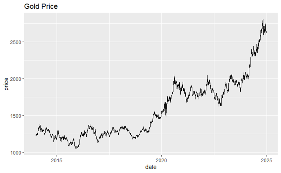
Figure 1: Daily gold price from 2014 to 2024 (photo credit: original)

3. Methodology and empirical analysis

3.1. Methodology

For a strong time-dependent series like the gold price, time-series ARIMA model is used to analysis this project.

According to Box and Jenkins, the ARIMA model seems to be one of the most used models for predicting the price of gold [7]. This approach makes an effort to guarantee that the future value of time series data maintains a useful relationship with both present and historical value. Foreign currency market analysts, importers, exporters, multinational corporations, speculators, and dealers all hold the view that historical trends can provide a short-term indication of future actions [8].

From a modeling, research perspective, The ARIMA model can not only be linked with many models such as GARCH and TGARCH to jointly discuss multiple aspects of a prediction problem. The former capturing volatility in the time series, and the latter focusing specifically on the asymmetry of volatility [9]. And the model can also be linked with machine training models, the most widely known is the Random Forest model, which can integrate the training of external factors affecting the model in addition to time, which greatly enhances the model's forecasting accuracy [10]. The research here starts with the most basic and simple ARIMA model.

The ARIMA model assumes that a variable's future value will be a linear function of several historical observations and random mistakes. In other words, the fundamental mechanism that creates the time series takes the following form:

\( {y_{t}}={θ_{0}}+{α_{1}}{y_{t-1}}+{α_{2}}{y_{t-2}}+⋯+{α_{p}}{y_{t-p}}+{δ_{1}}{ϵ_{t-1}}+{δ_{2}}{ϵ_{t-2}}+⋯+{δ_{q}}{ϵ_{t-q}} \) (1)

In this equation (1), \( {y_{t}} \) represents the actual value, and \( {ϵ_{t}} \) represents the random errors for each period.

Three iterative processes are part of the Box-Jenkins methodology: model identification, parameter estimate, and diagnostic checking [7].

3.2. Empirical analysis

Prior to the construction of the model, the data need to be preprocessed to check whether the series is stationary and whether it is a white noise series, only non-white noise stationary series have research value. The process starts with an ADF unit root test on the series.

Table 1: ADF test on the original data

According to the Table 1, the test's p-value is significantly higher than 0.05, meaning that the original hypothesis cannot be disproved at the 5% significance level. This indicates that the original series is non-stationary and that the trend must be eliminated by differentiating the data.

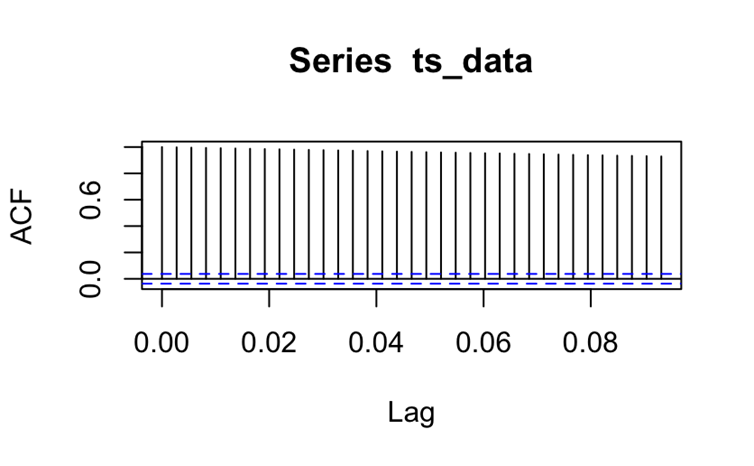
Figure 2: ACF plot from the original data (photo credit: original)

Additional evidence of sequence instability can also be provided by autocorrelation functions (ACF) and partial autocorrelation functions (PACF) (see Figure.2).

Table 2: ADF test on the one difference data

The results of the ADF test after one differencing of the original data are shown in the Table 2. The p-value becomes very small, and the original hypothesis can be rejected at the established significance level, and the series becomes stationary and can be analyzed at the next step. Here is basically certain that the difference can make the sequence to achieve a more ideal state, and the specific difference of several orders to be analyzed later to deal with.

Similarly, it is important to check whether the sequence is a white noise sequence, because the data of a white noise sequence is approximating a random wandering, and it would be pointless to study it. The Ljung-Box test was then applied to the data from the subsequent main differencing.

Table 3: Box-Ljung test on the one difference data

From the Ljung-box results (Table 3), it can be seen that the original hypothesis is rejected at the 5% level of significance, and it can be determined that the primary difference series is not a white noise series.

Table 4: Summary different model

After the data has been cleaned well it enters the modeling phase. First use the subset function to divide the data into the train set (2014/1/2-2021/1/4) and the test set (2021/1/5-2024/12/31), and after converting the set into time series data, use auto. Arima to select the optimal model parameters. Here, when using the auto. Arima instruction, the selection criteria for the functions are adjusted separately: that is, three different combinations of parameters are selected on the principle of AIC, BIC, and AICc minimization, respectively. The results are shown in the Table 4: two models, ARIMA (2, 1, 2) and ARIMA (0, 1, 0), were obtained. Either according to the principle of AIC, AICc minimization or economic intuition - the probability that the price of gold will be affected by the price of gold in a certain time interval in the past or by external factors - it is proved that ARIMA (2,1,2) performs better. This means that the absolute change in the current gold price (after differencing) is considered to be correlated with the change in the gold price in the previous two periods and the change in the error.

The forecast function is then used to generate a prediction set starting from 2021/1/4 with a length equal to the test set. And make two plots (Figure 3 and Figure 4) one alone for the prediction set (with confidence intervals) and the other comparing the real data (test set) curve with the prediction curve. It is important to note that the meaning of the horizontal coordinates of the two graphs is not the same, the former horizontal coordinate represents the order of the data (a total of 2,817 trading days of gold price data collected), the latter horizontal coordinate using a specific date.

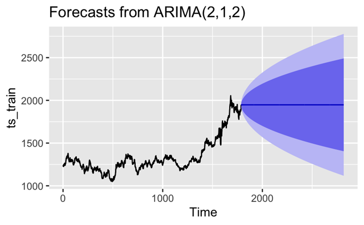
Figure 3: Forecast of ARIMA (2,1,2) (photo credit: original)

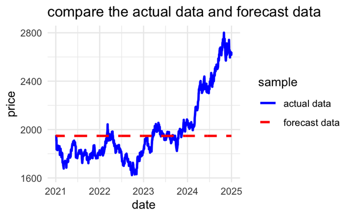
Figure 4: Comparing plot (photo credit: original)

3.3. Model checking

Based on the results, it was found that the prediction made by the set ARIMA model approximates a straight line. With such somewhat anomalous results, the model residuals need to be prioritized and tested to determine if the model is correct.

Table 5: Box-Ljung test on residuals from ARIMA (2,1,2)

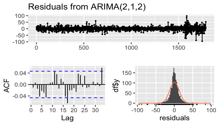
Figure 5: Residuals test (photo credit: original)

According to the Ljung-Box test (Table 5), the p-value of the model's residuals equal to 0.6572, a value greater than 0.05, which indicates that the residuals can basically be regarded as white noise at a significance level of 5%, in other words, there is no significant autocorrelation in the model's residuals. On the other hand, according to the distribution Figure 5, it can be seen that the residuals simultaneously satisfy the normal distribution. Therefore, it is basically certain that there is no significant structural or periodic information missing from the model and the residuals show random fluctuations.

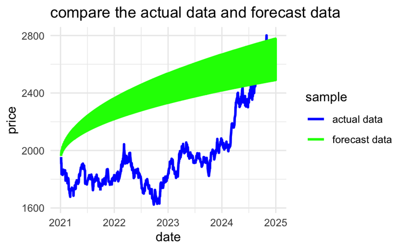
Figure 6: Prediction of the upper bound of the confidence interval (photo credit: original)

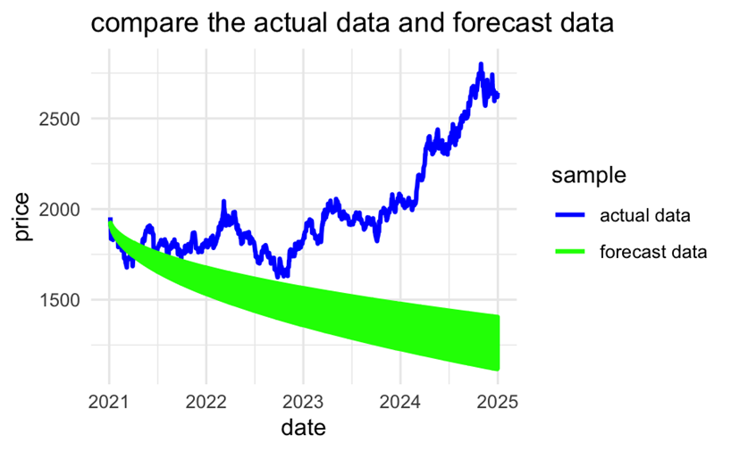
Figure 7: Prediction of the lowerbound of the confidence interval (photo credit: original)

To increase the evidence that the model was set up correctly, the upper and lower bounds of the confidence intervals of the ARIMA (2, 1, 2) predictions were plotted separately and it was observed whether the true values within the predicted years wandered within the confidence intervals. According to Figure 6 and Figure 7, it can be judged that the real data are basically predicted, and the prediction effect of the model can be accepted.

For the assessment of the model's prediction accuracy (Table 4), three metrics are focused on: the RMSE, MAE, and MAPE, which represent the root mean square error, the mean absolute error, and the mean absolute percent error, respectively. The dependent variable studied in this research is the price of gold, which is a variable in thousands, so based on the RMSE (13.0274), MAE (8.7428), and MAPE (0.6388%) of this model, it can be concluded that the model's prediction error is relatively small [11].

4. Discussion

For the prediction curve to be a horizontal straight line of size approximately equal to the last training point, it is analyzed in two ways.

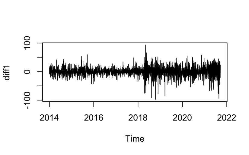
Figure 8: Preview of the data after one difference (photo credit: original)

Interpreted from the model point of view, the first point is that after one difference, the sequence data becomes a stationary sequence, that is to say, the data before the difference has a unit root characteristic, and its characteristic is approximated to random wandering (Figure 8) [12]. And for the random wandering sequence, its optimal prediction value is the current value or the average value in the long term. Another point is that the ARIMA model is less capable of capturing long-term fluctuations, and its long-term prediction results will basically be stabilized at the current value.

From an economic point of view, the forecast results of this study basically confirm the efficient market hypothesis. For a highly liquid and highly placed financial asset such as gold, there is a very high degree of information transparency about its price, while participants in this market have sufficient incentives to obtain information. Therefore, the current price of gold has already reflected all the information available at present, and how the price of gold changes in the future depends on how the information changes in the future, that is to say, it is difficult for ARIMA to accurately predict the long term by using only seven years of historical data on the price of gold.

In summary, it may be able to gain some insights on the policy front. In order to avoid drastic fluctuation of gold price in the long term and affect the domestic financial market, on the one hand, the government should enhance the transparency of information, on the other hand, the government should take active monetary policy macro-control to stabilize the price.

5. Conclusion

The purpose of this study is to determine the forecasting effect of ARIMA model and to forecast the future price of gold. Using daily data from 2014 to 2024 and with RStudio software, the best ARIMA model parameters (2, 1, 2) were fitted to find out the best ARIMA model for the gold price and the predicted future price curve is basically a straight line with a magnitude equal to the last observation. Such results basically confirm the efficient market hypothesis. Although the predictions of the model are different from expectations, testing the model residuals and MSE and RMSE proves that the model is not set up incorrectly, which gives many insights for subsequent studies.

The model determined in this study is valid only under stable market, and the results of this study should not be valid when the market fluctuates due to some unexpected events. On the one hand, it is obvious that the training set divided in this study does not capture the abnormal upward trend after 2021, which leads to an incomplete model. On the other hand, the price of gold is a very complex proposition that is affected by many external factors. To make the model perform better, machine learning models (Random Forest, LSTM) can be introduced in the future to capture the unquantifiable external influences, thus enhancing the model's interpretability for different economic scenarios.

References

[1]. Abdullah, L. (2012). ARIMA model for gold bullion coin selling prices forecasting. International Journal of Advances in Applied Sciences, 1(4), 153-158.
[2]. Gaspareniene, L., Remeikiene, R., Sadeckas, A., & Ginevicius, R. (2018). The main gold price determinants and the forecast of gold price future trends. Economics & Sociology, 11(3), 248-264.
[3]. Bunnag, T. (2024). The Importance of Gold’s Effect on Investment and Predicting the World Gold Price Using the ARIMA and ARIMA-GARCH Model. Ekonomikalia Journal of Economics, 2(1), 38-52.
[4]. Makala, D., & Li, Z. (2021, February). Prediction of gold price with ARIMA and SVM. In Journal of Physics: Conference Series (Vol. 1767, No. 1, p. 012022). IOP Publishing.
[5]. Demirezen, S. (2021). Forecasting of Gold Prices with ARIMA and Random Forest Regression and Evaluating of Their Prediction Performance. SSRJ| Social Sciences Research Journal| Online ISSN: 2147-5237, 10(03), 747-758.
[6]. Noureen, S., Atique, S., Roy, V., & Bayne, S. (2019). A comparative forecasting analysis of arima model vs random forest algorithm for a case study of small-scale industrial load. International Research Journal of Engineering and Technology, 6(09), 1812-1821.
[7]. Box, G. (2013). Box and Jenkins: time series analysis, forecasting and control. In A Very British Affair: Six Britons and the Development of Time Series Analysis During the 20th Century (pp. 161-215). London: Palgrave Macmillan UK.
[8]. Yang, X. (2019, January). The prediction of gold price using ARIMA model. In 2nd International Conference on Social Science, Public Health and Education (SSPHE 2018) (pp. 273-276). Atlantis Press.
[9]. Yaziz, S. R., Azizan, N. A., Ahmad, M. H., & Zakaria, R. (2016). Modelling gold price using ARIMA-TGARCH. Applied Mathematical Sciences, 10(28), 1391-1402.
[10]. Tyralis, H., & Papacharalampous, G. (2017). Variable selection in time series forecasting using random forests. Algorithms, 10(4), 114.
[11]. Azan, A. N. A. M., Mototo, N. F. A. M. Z., & Mah, P. J. W. (2021). The Comparison between ARIMA and ARFIMA model to forecast kijang emas (gold) prices in Malaysia using MAE, RMSE and MAPE. Journal of Computing Research and Innovation, 6(3), 22-33.
[12]. Kuo, H. H. (2018). White noise distribution theory. CRC press.
Cite this article
Wang,Z. (2025). The Effectiveness of Forecasting Gold Prices Using ARIMA Models. Advances in Economics, Management and Political Sciences,185,232-241.
Data availability
The datasets used and/or analyzed during the current study will be available from the authors upon reasonable request.
Disclaimer/Publisher's Note
The statements, opinions and data contained in all publications are solely those of the individual author(s) and contributor(s) and not of EWA Publishing and/or the editor(s). EWA Publishing and/or the editor(s) disclaim responsibility for any injury to people or property resulting from any ideas, methods, instructions or products referred to in the content.
About volume
Volume title: Proceedings of ICEMGD 2025 Symposium: Innovating in Management and Economic Development
© 2024 by the author(s). Licensee EWA Publishing, Oxford, UK. This article is an open access article distributed under the terms and
conditions of the Creative Commons Attribution (CC BY) license. Authors who
publish this series agree to the following terms:
1. Authors retain copyright and grant the series right of first publication with the work simultaneously licensed under a Creative Commons
Attribution License that allows others to share the work with an acknowledgment of the work's authorship and initial publication in this
series.
2. Authors are able to enter into separate, additional contractual arrangements for the non-exclusive distribution of the series's published
version of the work (e.g., post it to an institutional repository or publish it in a book), with an acknowledgment of its initial
publication in this series.
3. Authors are permitted and encouraged to post their work online (e.g., in institutional repositories or on their website) prior to and
during the submission process, as it can lead to productive exchanges, as well as earlier and greater citation of published work (See
Open access policy for details).